Vehicle routing problem

Setting up the problem

The VRP concerns the service of a delivery company. How things are delivered from one or more depots which has a given set of home vehicles and operated by a set of drivers who can move on a given road network to a set of customers. It asks for a determination of a set of routes, S, (one route for each vehicle that must start and finish at its own depot) such that all customers' requirements and operational constraints are satisfied and the global transportation cost is minimized. This cost may be monetary, distance or otherwise.

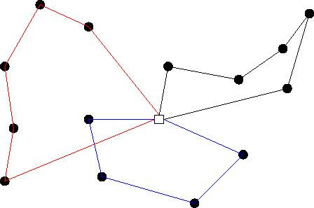
The road network can be described using a graph where the arcs are roads and vertices are junctions between them. The arcs may be directed or undirected due to the possible presence of one way streets or different costs in each direction. Each arc has an associated cost which is generally its length or travel time which may be dependent on vehicle type.

To know the global cost of each route, the travel cost and the travel time between each customer and the depot must be known. To do this our original graph is transformed into one where the vertices are the customers and depot, and the arcs are the roads between them. The cost on each arc is the lowest cost between the two points on the original road network. This is easy to do as shortest path problems are relatively easy to solve. This transforms the sparse original graph into a complete graph. For each pair of vertices i and j, there exists an arc (i,j) of the complete graph whose cost is written as C i j and is defined to be the cost of shortest path from i to j. The travel time t i j is the sum of the travel times of the arcs on the shortest path from i to j on the original road graph.

Sometimes it is impossible to satisfy all of a customer's demands and in such cases solvers may reduce some customers' demands or leave some customers unserved. To deal with these situations a priority variable for each customer can be introduced or associated penalties for the partial or lack of service for each customer given

The objective function of a VRP can be very different depending on the particular application of the result but a few of the more common objectives are:

VRP variants

Several variations and specializations of the vehicle routing problem exist:

Several software vendors have built software products to solve the various VRP problems. Numerous articles are available for more detail on their research and results.

Although VRP is related to the Job Shop Scheduling Problem, the two problems are typically solved using different techniques.

Exact solution methods

There are three main different approaches to modelling the VRP

1. Vehicle flow formulations—this uses integer variables associated with each arc that count the number of times that the edge is traversed by a vehicle. It is generally used for basic VRPs. This is good for cases where the solution cost can be expressed as the sum of any costs associated with the arcs. However it can't be used to handle many practical applications.
2. Commodity flow formulations—additional integer variables are associated with the arcs or edges which represent the flow of commodities along the paths travelled by the vehicles. This has only recently been used to find an exact solution.
3. Set partitioning problem—These have an exponential number of binary variables which are each associated with a different feasible circuit. The VRP is then instead formulated as a set partitioning problem which asks what is the collection of circuits with minimum cost that satisfy the VRP constraints. This allows for very general route costs.

Vehicle flow formulations

The formulation of the TSP by Dantzig, Fulkerson and Johnson was extended to create the two index vehicle flow formulations for the VRP

min ∑ i ∈ V ∑ j ∈ V c i j x i j

subject to

∑ i ∈ V x i j = 1 ∀ j ∈ V ∖ { 0 } ; ( 1 ) ∑ j ∈ V x i j = 1 ∀ i ∈ V ∖ { 0 } ; ( 2 ) ∑ i ∈ V x i 0 = K ; ( 3 ) ∑ j ∈ V x 0 j = K ; ( 4 ) ∑ i ∉ S ∑ j ∈ S x i j ≥ r ( S ) ∀ S ⊆ V ∖ { 0 } , S ≠ ∅ ; ( 5 ) x i j ∈ { 0 , 1 } ∀ i , j ∈ V . ( 6 )

Constraints 1 and 2 state that exactly one arc enters and exactly one leaves each vertex associated with a customer, respectively. Constraints 3 and 4 say that the number of vehicles leaving the depot is the same as the number entering. Constraints 5 are the capacity cut constraints, which impose that the routes must be connected and that the demand on each route must not exceed the vehicle capacity. Finally, constraints 6 are the integrality constraints.

One arbitrary constraint among the 2|V| constraints is actually implied by the remaining 2|V|-1 ones so it can be removed. Each cut defined by a customer set S is crossed by a number of arcs not smaller than r(s) (minimum number of vehicles needed to serve set S).

An alternative formulation may be obtained by transforming the capacity cut constraints into generalised subtour elimination constraints (GSECs). ∑ i ∈ S ∑ j ∈ S x i j ≤ | S | − r ( s ) which imposes that at least r(s) arcs leave each customer set S.

GCECs and CCCs have an exponential number of constraints so it is practically impossible to solve the linear relaxation. A possible way to solve this is to consider a limited subset of these constraints and add the rest if needed.

A different method again is to use a family of constraints which have a polynomial cardinality which are known as the MTZ constraints, they were first proposed for the TSP and subsequently extended by Christofides, Mingozzi and Toth. u i − u j + C x i j ≤ C − d j             ∀ i , j ∈ V ∖ { 0 } , i ≠ j         s.t.  d i + d j ≤ C

d i ≤ u i ≤ C             ∀ i ∈ V ∖ { 0 }

where u i ,   i ∈ V ∖ { 0 } is an additional continuous variable which represents the load of the vehicle after visiting customer i and d_i is the demand of customer i. These impose both the connectivity and the capacity requirements. When x i j = 0 constraint then i 'is not binding' since u i ≤ C and u j ≥ d j whereas x i j = 1 they impose that u j ≥ u i + d j .

These have been used extensively to model the basic VRP (CVRP) and the VRPB. However their power is limited to these simple problems. They can only be used when the cost of the solution can be expressed as the sum of the costs of the arc costs. We cannot also know which vehicle traverses each arc. Hence we cannot use this for more complex models where the cost and or feasibility is dependent on the order of the customers or the vehicles used.

Manual vs. Automatic Optimum Routing

There are many methods how to solve vehicle routing problem manually. For example, optimum routing is a big efficiency issue for forklifts in large warehouses. Some of the manual methods to decide upon the most efficient route are: Largest gap, S-shape, Aisle-by-aisle, Combined and Combined +. While Combined + method is the most complex, thus the hardest to be used by lift truck operators, it is the most efficient routing method. Still the percentage difference between the manual optimum routing method and the real optimum route was on average 13%.