Variance based sensitivity analysis

Decomposition of Variance

From a black box perspective, any model may be viewed as a function Y=f(X), where X is a vector of d uncertain model inputs {X₁, X₂, ... X_d}, and Y is a chosen univariate model output (note that this approach examines scalar model outputs, but multiple outputs can be analysed by multiple independent sensitivity analyses). Furthermore, it will be assumed that the inputs are independently and uniformly distributed within the unit hypercube, i.e. X i ∈ [ 0 , 1 ] for i = 1 , 2 , . . . , d . This incurs no loss of generality because any input space can be transformed onto this unit hypercube. f(X) may be decomposed in the following way,

where f₀ is a constant and f_i is a function of X_i, f_ij a function of X_i and X_j, etc. A condition of this decomposition is that,

i.e. all the terms in the functional decomposition are orthogonal. This leads to definitions of the terms of the functional decomposition in terms of conditional expected values,

From which it can be seen that f_i is the effect of varying X_i alone (known as the main effect of X_i), and f_ij is the effect of varying X_i and X_j simultaneously, additional to the effect of their individual variations. This is known as a second-order interaction. Higher-order terms have analogous definitions.

Now, further assuming that the f(X) is square-integrable, the functional decomposition may be squared and integrated to give,

Notice that the left hand side is equal to the variance of Y, and the terms of the right hand side are variance terms, now decomposed with respect to sets of the X_i. This finally leads to the decomposition of variance expression,

where

and so on. The X_~i notation indicates the set of all variables except X_i. The above variance decomposition shows how the variance of the model output can be decomposed into terms attributable to each input, as well as the interaction effects between them. Together, all terms sum to the total variance of the model output.

First-order indices

A direct variance-based measure of sensitivity S_i, called the "first-order sensitivity index", or "main effect index" is stated as follows,

This is the contribution to the output variance of the main effect of X_i, therefore it measures the effect of varying X_i alone, but averaged over variations in other input parameters. It is standardised by the total variance to provide a fractional contribution. Higher-order interaction indices S_ij, S_ijk and so on can be formed by dividing other terms in the variance decomposition by Var(Y). Note that this has the implication that,

Total-effect index

Using the S_i, S_ij and higher-order indices given above, one can build a picture of the importance of each variable in determining the output variance. However, when the number of variables is large, this requires the evaluation of 2^d-1 indices, which can be too computationally demanding. For this reason, a measure known as the "Total-effect index" or "Total-order index", S_Ti, is used. This measures the contribution to the output variance of X_i, including all variance caused by its interactions, of any order, with any other input variables. It is given as,

Note that unlike the S_i,

due to the fact that the interaction effect between e.g. X_i and X_j is counted in both S_Ti and S_Tj In fact, the sum of the S_Ti will only be equal to 1 when the model is purely additive.

Calculation of indices

For analytically tractable functions, the indices above may be calculated analytically by evaluating the integrals in the decomposition. However, in the vast majority of cases they are estimated - this is usually done by the Monte Carlo method.

Sampling sequences

The Monte Carlo approach involves generating a sequence of randomly distributed points inside the unit hypercube (strictly speaking these will be pseudorandom). In practice, it is common to substitute random sequences with low-discrepancy sequences to improve the efficiency of the estimators. This is then known as the Quasi-Monte Carlo method. Some low-discrepancy sequences commonly used in sensitivity analysis include the Sobol sequence and the Latin hypercube design.

Procedure

To calculate the indices using the (Quasi) Monte Carlo method, the following steps are used:

1. Generate an Nx2d sample matrix, i.e. each row is a sample point in the hyperspace of 2d dimensions. This should be done with respect to the probability distributions of the input variables.
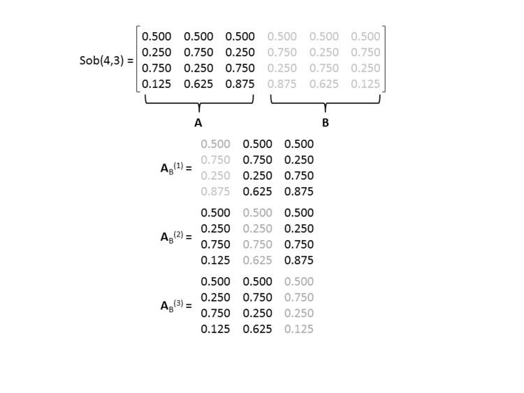
2. Use the first d columns of the matrix as matrix A, and the remaining d columns as matrix B. This effectively gives two independent samples of N points in the d-dimensional unit hypercube.
3. Build d further Nxd matrices A_Bⁱ, for i = 1,2,...,d, such that the ith column of A_Bⁱ is equal to the ith column of B, and the remaining columns are from A.
4. The A, B, and the d A_Bⁱ matrices in total specify N(d+2) points in the input space (one for each row). Run the model at each design point in the A, B, and A_Bⁱ matrices, giving a total of N(d+2) model evaluations - the corresponding f(A), f(B) and f(A_Bⁱ) values.
5. Calculate the sensitivity indices using the estimators below.

The accuracy of the estimators is of course dependent on N. The value of N can be chosen by sequentially adding points and calculating the indices until the estimated values reach some acceptable convergence. For this reason, when using low-discrepancy sequences, it can be advantageous to use those that allow sequential addition of points (such as the Sobol sequence), as compared to those that do not (such as Latin hypercube sequences).

Estimators

There are a number of possible Monte Carlo estimators available for both indices. Two that are currently in general use are,

and

for the estimation of the S_i and the S_Ti respectively.

Computational Expense

For the estimation of the S_i and the S_Ti for all input variables, N(d+2) model runs are required. Since N is often of the order of hundreds or thousands of runs, computational expense can quickly become a problem when the model takes a significant amount of time for a single run. In such cases, there are a number of techniques available to reduce the computational cost of estimating sensitivity indices, such as emulators, HDMR and FAST.