Trigonometry in Galois fields

Trigonometry over a Galois field

The set GI(q) of Gaussian integers over the finite field GF(q) plays an important role in the trigonometry over finite fields. If q = p^r is a prime power such that −1 is a quadratic non-residue in GF(q), then GI(q) is defined as

GI(q) = {a + jb; a, b ∈ GF(q)},

where j is a symbolic square root of −1 (that is j is defined by j² = −1). Thus GI(q) is a field isomorphic to GF(q²).

Trigonometric functions over the elements of a Galois field can be defined as follows:

Let ζ be an element of multiplicative order N in GI(q), q = p^r, p an odd prime such that p  ≡ 3 (mod 4). The GI(q)-valued k-trigonometric functions of ( ∠ ζ i ) in GI(q) (by analogy, the trigonometric functions of k times the "angle" of the "complex exponential" ζ ⁱ) are defined as

cos k ⁡ ( ∠ ζ i ) = ( 2 − 1 mod p ) ⋅ ( ζ i k + ζ − i k ) , sin k ⁡ ( ∠ ζ i ) = ( 1 / j ) ( 2 − 1 mod p ) ⋅ ( ζ i k − ζ − i k ) ,

for i, k = 0, 1,...,N − 1. We write cos_k( ∠ ζ ⁱ) and sin_k ( ∠ ζ ⁱ) as cos_k(i) and sin_k(i), respectively. The trigonometric functions above introduced satisfy properties P1-P12 below, in GI(p).

P1. Unit circle: sin k 2 ⁡ ( i ) + cos k 2 ⁡ ( i ) ≡ 1.

P2. Even/Odd:

cos k ⁡ ( i ) ≡ cos k ⁡ ( − i ) .

sin k ⁡ ( i ) ≡ − sin k ⁡ ( − i ) .

P3. Euler formula: ζ k i ≡ cos k ⁡ ( i ) + j sin k ⁡ ( i ) .

P4. Addition of arcs:

cos k ⁡ ( i + t ) ≡ cos k ⁡ ( i ) cos k ⁡ ( t ) − sin k ⁡ ( i ) sin k ⁡ ( t ) ,

sin k ⁡ ( i + t ) ≡ sin k ⁡ ( i ) cos k ⁡ ( t ) + sin k ⁡ ( t ) cos k ⁡ ( i ) .

P5. Double arc:

cos k 2 ⁡ ( i ) ≡ ( 2 − 1 mod p ) ⋅ ( 1 + cos k ⁡ ( 2 i ) ) ,

sin k 2 ⁡ ( i ) ≡ ( 2 − 1 mod p ) ⋅ ( 1 − cos k ⁡ ( 2 i ) .

P6. Symmetry:

cos k ⁡ ( i ) ≡ cos i ⁡ ( k ) ,

sin k ⁡ ( i ) ≡ sin i ⁡ ( k ) .

P7. Complementary symmetry: with ( k + t ) = ( i + r ) = N ,

cos k ⁡ ( i ) ≡ cos r ⁡ ( t ) ,

sin k ⁡ ( i ) ≡ sin r ⁡ ( t ) .

P8. Periodicity:

cos k ⁡ ( i + N ) ≡ cos k ⁡ ( i ) ,

sin k ⁡ ( i + N ) ≡ sin k ⁡ ( i ) .

P9. Complement: with ( i + t ) = N ,

cos k ⁡ ( i ) ≡ cos k ⁡ ( t ) ,

sin k ⁡ ( i ) ≡ − sin k ⁡ ( t ) .

P10. cos k ⁡ ( i ) summation: ∑ k = 0 N − 1 cos k ⁡ ( i ) ≡ .

P11. sin k ⁡ ( i ) summation: ∑ k = 0 N − 1 sin k ⁡ ( i ) ≡ 0.

P12. Orthogonality: ∑ k = 0 N − 1 [ cos k ⁡ ( i ) sin k ⁡ ( t ) ] ≡ 0.

Examples

With ζ = 3, a primitive element of GF(7), then cos_k(i) and sin_k(i) functions take the following values in GI(7):

Let ζ = j, an element of order 4 in GI(3). The cos_k(i) and sin_k(i) functions take the following values in GI(3):

Unimodular groups

The unimodular set of GI(p), denoted by G₁, is the set of elements ζ = (a + jb) ∈ GI(p), such that a² + b² ≡ 1 (mod p).

To determine the elements of the unimodular group it helps to observe that if ζ = a + jb is one such element, then so is every element in the set ζ = {b + ja, (p − a) + jb, b + j(p − a), a +j(p − b), (p − b) + ja, (p − a) + j(p − b), (p − b) + j(p − a)}.

Example

Unimodular groups of GF(7²) and GF(11²). In each case, table III lists the elements of the subgroups G₁ of order 8 and 12, and their orders.

Figure 1 illustrates the 12 roots of unity in GF(11²). Clearly, G₁ is isomorphic to C12, the group of proper rotations of a regular dodecagon. ζ =8+j6 is a group generator corresponding to a counter-clockwise rotation of 2π/12 = 30°. Symbols of the same colour indicate elements of same order, which occur in conjugate pairs.

Polar form

Let G_r and G_θ be subgroups of the multiplicative group of the nonzero elements of GI(p), of orders (p − 1)/2 and 2(p + 1), respectively. Then all nonzero elements of GI(p) can be written in the form ζ = α·β, where α ∈ G_r and β ∈ G_θ.

Considering that any element of a cyclic group can be written as an integral power of a group generator, it is possible to set r = α and ε^θ = β, where ε is a generator of G θ . The powers ε^θ of this element play the role of e^jθ over the complex field. Thus, the polar representation assumes the desired form, ζ = r ⋅ ϵ θ , where r plays the role of the modulus of ζ. Therefore, it is necessary to define formally the modulus of an element in a finite field. Considering the nonzero elements of GF(p), it is a well-known fact that half of them are quadratic residues of p. The other half, those that do not possess square root, are the quadratic non-residue (in the field of real numbers, the elements are divided into positive and negative numbers, which are, respectively, those that possess and do not possess a square root).

The standard modulus operation (absolute value) in R always gives a positive result.

By analogy, the modulus operation in GF(p) is such that it always results in a quadratic residue of p.

The modulus of an element a ∈ G F ( p ) , where p = 4k + 3, is

| a | = { a , if a ( p − 1 ) / 2 ≡ 1 mod p , − a , if a ( p − 1 ) / 2 ≡ − 1 mod p .

The modulus of an element of GF(p) is a quadratic residue of p.

The modulus of an element a + jb ∈ GI(p), where p = 4k + 3, is

∣ a + j b ∣= | ∣ a 2 + b 2 ∣ | .

In the continuum, such expression reduces to the usual norm of a complex number, since both, a² + b² and the square root operation, produce only nonnegative numbers.

The group of modulus of GI(p), denoted by G_r, is the subgroup of order (p − 1)/2 of GI(p).

The group of phases of GI(p), denoted by G _θ , is the subgroup of order 2(p + 1) of GI(p).

An expression for the phase θ as a function of a and b can be found by normalising the element ζ (that is, calculating ζ / r = ϵ θ ), and then solving the discrete logarithm problem of ζ /r in the base ϵ over GF(p). Thus, the conversion rectangular to polar form is possible.

The similarity with the trigonometry over the field of real numbers is now evident: the modulus belongs to GF(p) (the modulus is a real number) and is a quadratic residue (a positive number), and the exponential component ϵ ^θ ) has modulus one and belongs to GI(p) (e ^{j θ} also has modulus one and belongs to the complex field C ).

The Z plane in a Galois field

The complex Z plane (Argand diagram) in GF(p) can be constructed from the supra-unimodular set of GI(p):

The supra-unimodular set of GI(p), denoted G_s, is the set of elements ζ = (a + jb) ∈ GI(p), such that (a² + b²) ≡ −1 (mod p).

The structure <G_s,*>, is a cyclic group of order 2(p + 1), called the supra-unimodular group of GI(p).

The elements ζ = a + jb of the supra-unimodular group G_s satisfy (a² + b²)² ≡ 1 (mod p) and all have modulus 1. G_s is precisely the group of phases G θ .

If p is a Mersenne prime (p = 2ⁿ − 1, n > 2), the elements ζ = a + jb such that a² + b² ≡ −1 (mod p) are the generators of G_s.

Examples

Let p = 31, a Mersenne prime, and ζ = 6 + j16. Then r = | ( | 6 2 + 16 2 | ) | ≡ | | 13 | | ≡ 7 (mod 31), so that ϵ = ζ /r = 23 + j20 and a² + b² = 23² + 20² ≡ −1 (mod 31). Therefore ε has order 2(p + 1) = 64 (a generator). A unimodular element β of order N, such that N | 25, can be found taking β = ϵ ^2(p+1)/N = ϵ 64 / N .

The Z plane in GF(7): With p = 7, and ζ = 6 + j4, r = | ( | 6 2 + 4 2 | ) | ≡ | | 3 | | ≡ 2 (mod 31), so that ε = ζ/r = 3 + j2 and a² + b² = 13 ≡ −1 (mod 31). Therefore ε has order 2(p + 1) = 16, so it is a generator of the group G_s.

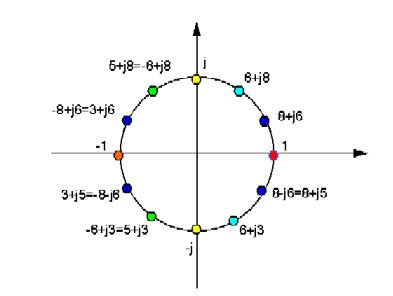
A generator ε of the supra-unimodular group is used to construct the Z plane over GF(p). The Z plane over GF(7) is depicted in figure 2. There are 2(p + 1) = 16 elements in each circle. The nonzero elements, namely ±1, ±2, ±3, are located on the horizontal axis, in the right or left side, according if they are, respectively, quadratic residues (QR) or quadratic non-residues (NQR) of p = 7. There are three circles, of radius 1, 2 and 4, corresponding to the (p − 1)/2 = 3 elements of the group of modules G_r. A similar situation occurs for the elements of GI(7) of the form jb. The 16 elements on the unit circle correspond to the elements of G_s and are obtained as powers of ε. The even powers correspond to the elements of G₁ (a² + b² ≡ 1 (mod 7)) and the odd powers to the elements satisfying a² + b² ≡ −1 (mod 7). The remaining 32 elements of the Z plane are obtained simply by multiplying those on the unit circle by the modulus 2 and 4. The elements on the straight line y=±x over a finite field also possesses the usual interpretation associated with tg  θ = ±1.

The number of elements of a given order as elements of GI(7) in the z plane over GF(7) is given in the inset of figure 2.

Back to the GF(p)-trigonometry

In the above, if the choice of ζ is careless, the trigonometric functions may possibly be complex, i.e., they may be GI(p)-valued. However, if ζ =a+jb is chosen to be a unimodular element, so that a²+b² ≡ 1 (mod p), then cos(.) and sin(.) are GF(p)-valued. With that in mind and dropping a few subscripts, the definitions may be rephrased in a simpler form as:

cos ⁡ ( i ) = ( 2 − 1 mod p ) ⋅ ( ϵ i + ϵ − i ) ,

sin ⁡ ( i ) = ( 1 / j ) ( 2 − 1 mod p ) ⋅ ( ϵ i − ϵ − i ) ,

for i = 0, 1, ..., p. The k subscript in the earlier definition gives an unexpected two-dimensional character to the cos(.) and sin(.) functions. As a matter of fact, it means only that to compute the entries in tables I and II, a different value of ϵ = ζ ^k was used for each k. These k-trigonometric functions lead to sequences with interesting orthogonality properties which may be used to construct new finite field transforms.

Now, to play with a trigonometry over GF(7) on the unit circle, it seems much more natural to use, for instance, ϵ = 2 + j2 ∈ GI(7), instead of ζ = 3 ∈ GF(7) as in table I (examples). In this case, | ϵ | = 1 and both cos and sin are "real-valued" functions, as expected.

Further, if ϵ is chosen from the set of unimodular elements, it can be shown that the "real" part of ϵ i is equal to the "real" part of ϵ − i , and the "imaginary" part of ϵ i is equal to the negative of the "imaginary" part of ϵ − i . So, for unimodular element ϵ , the definitions simplify to:

cos ⁡ ( i ) = R e { ϵ i }

sin ⁡ ( i ) = I m { ϵ i }

Example

With ϵ = 2 + j2, a unimodular element of order p + 1 = 8 of GI(7), the cos(i) and sin(i) functions take the following values in GF(7):

Trajectories over the Galois Z plane in GF(p)

When calculating the order of a given element, the intermediate results generate a trajectory on the Galois Z plane, called the order trajectory. In particular, If ζ has order N, the trajectory goes through N distinct points on the Z plane, moving in a pattern that depends on N. Specifically, the order trajectory touches on every circle of the Galois Z plane (there are ||G_r|| of them), in order of increasing modulus, always returning to the unit circle. If it starts on a given radius, say R, it will visit, counter-clockwise, every radius of the form R+k.r, where r=(p²−1)/N and k = 0, 1, 2, ....., N − 1. Given a prime p  ≡  3 (mod 4), there are a (finite) number of (p − 1)/2 distinct circles over the Galois Z plane GI(p), and the number of distinct finite field ellipses is (p − 1).(p − 3)/4.

Table V lists some elements ζ ∈ GI(7) and their orders N. Figures 3–5 show the order trajectories generated by ζ.