Time varying network

Applicability

Time-varying networks are inherently dynamic, and used for modeling spreading processes on networks. Whether using time-varying networks will be worth the added complexity depends on the relative time scales in question. Time-varying networks are most useful in describing systems where the spreading process on a network and the network itself evolve at similar timescales.

Let the characteristic timescale for the evolution of the network be t N , and the characteristic timescale for the evolution of the spreading process be t P . A process on a network will fall into one of three categories:

Static approximation – where t N ≫ t P . The network evolves relatively slowly, so the dynamics of the process can be approximated using a static version of the network.

Time-varying network – where t N ∼ t P . The network and the process evolve at comparable timescales so the interplay between them becomes important.

Annealed approximation – where t N ≪ t P . The network evolves relatively rapidly, so the dynamics of the process can be approximated using a time averaged version of the network.

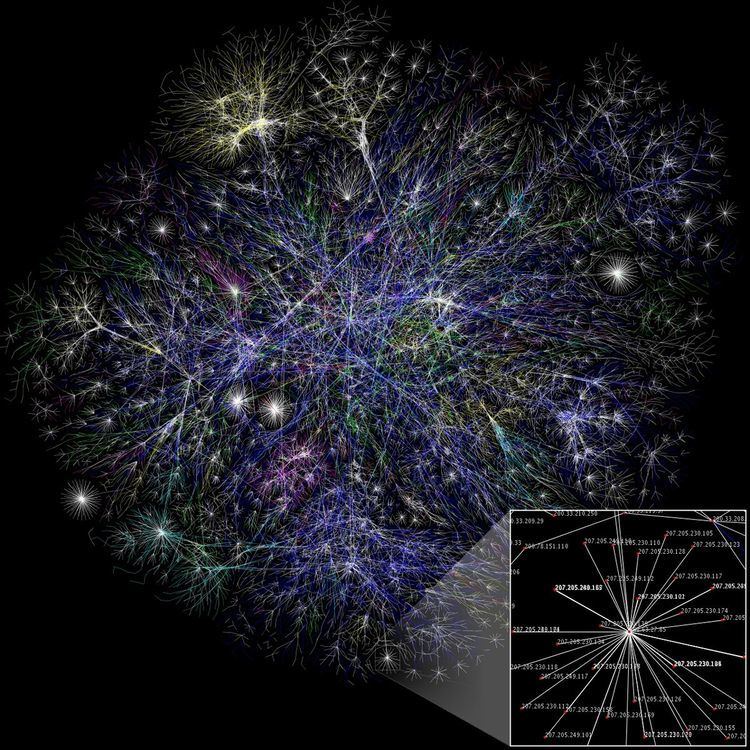
The flow of data over the internet is an example for the first case, where the network changes very little in the fraction of a second it takes for a network packet to traverse it. The spread of sexually transmitted diseases is an example of the second, where the prevalence of the disease spreads in direct correlation to the rate of evolution of the sexual contact network itself. Behavioral contagion is an example of the third case, where behaviors spread through a population over the combined network of many day-to-day social interactions.

Representations

There are three common representations for time-varying network data.

Contact sequences – if the duration of interactions are negligible, the network can be represented as a set C of contacts ( i , j , t ) where i and j are the nodes and t the time of the interaction. Alternatively, it can be represented as an edge list E where each edge e is a pair of nodes and has a set of active times T e = { t 1 , … , t n } .

Interval graphs – if the duration of interactions are non-negligible, T e becomes a set of intervals over which the edge e is active. T e = { ( t 1 , t 1 ′ ) , … , ( t n , t n ′ ) }

Snapshots – time-varying networks can also be represented as a series of static networks, one for each time step.

Properties

The measures used to characterize static networks are not immediately transferable to time-varying networks. See Path, Connectedness, Distance, Centrality. However, these network concepts have been adapted to apply to time-varying networks.

Time respecting paths

Time respecting paths refers to the sequences of links that can be traversed in a time-varying network under the constraint that the next link to be traversed is activated at some point after the current one. Like in a directed graph, a path from i to j does not mean there is a path from j to i . In contrast to paths in static and evolving networks, however, time respecting paths are also non-transitive. That is to say, just because there is a path from i to j and from j to k does not mean that there is a path from i to k . Furthermore, time respecting paths are themselves time-varying, and are only valid paths during a specific time interval.

Reachability

While analogous to connectedness in static networks, reachability is a time-varying property best defined for each node in the network. The set of influence of a node i is the set of all nodes that can be reached from i via time respecting paths, note that it is dependent on the start time t . The source set of a node i is the set of all nodes that can reach i via time respecting paths within a given time interval. The reachability ratio can be defined as the average over all nodes i of the fraction of nodes within the set of influence of i .

Connectedness of an entire network is less conclusively defined, although some have been proposed. A component may be defined as strongly connected if there is a directed time respecting path connecting all nodes in the component in both directions. A component may be defined as weakly connected if there is an undirected time respecting path connecting all nodes in the component in both directions. Also, a component may be defined as transitively connected if transitivity holds for the subset of nodes in that component.

Latency

Also called temporal distance, latency is the time-varying equivalent to distance. In a time-varying network any time respecting path has a duration, namely the time it takes to follow that path. The fastest such path between two nodes is the latency, note that it is also dependent on the start time. The latency from node i to node j beginning at time t is denoted by λ i , t ( j ) .

Centrality measures

Measuring centrality on time-varying networks involves a straightforward replacement of distance with latency. For discussions of the centrality measures on a static network see Centrality.

Closeness centrality is large for nodes i that are close to all other nodes (i.e. have small latency λ i ( j ) for all j )

Betweenness centrality is large for nodes that are often a part of the smallest latency paths between other pairs of nodes. It is defined as the ratio of the number of smallest latency paths from j and k that pass through i to the total number of smallest latency paths from j and k

The time-varying nature of latency, specifically that it will become infinity for all node pairs as the time approaches the end of the network interval used, makes an alternative measure of closeness useful. Efficiency uses instead the reciprocal of the latency, so the efficiency approaches zero instead of diverging. Higher values for efficiency correspond to more central nodes in the network.

Temporal patterns

Time-varying network allow for analysis of explicit time dependent properties of the network. It is possible to extract recurring and persistent patterns of contact from time-varying data in many ways. This is an area of ongoing research.

Characteristic times of the system can be found by looking for distinct changes in a variable, such as the reachability ratio. For example, if one allows only a finite waiting time at all nodes in calculating latency, one can find interesting patterns in the resulting reachability ratio. For a mobile call network, the reachability ratio has been found to increase dramatically if one allows delays of at least two days, and for the airline network the same effect has been found at around 30 minutes.

Persistent patterns are ones that reoccur frequently in the system. They can be discovered by averaging over different Δ t across the time interval of the system and looking for patterns that reoccur over a specified threshold.

Motifs are specific temporal patterns that occur more often the expected in a system. The time-varying network of Facebook wall postings, for example, has higher frequency of chains, stars, and back and forth interactions that could be expected for a randomized network.

Dynamics

Time-varying networks allow for the analysis of an entirely new dimension of dynamic processes on networks. In cases where the time scales of evolution of the network and the process are similar, the temporal structure of time-varying networks has a dramatic impact on the spread of the process over the network.

Burstiness

The time between two consecutive events, for an individual node or link, is called the inter-event time. The distribution of inter-event times of a growing number of important, real-world, time-varying networks have been found to be bursty, meaning inter-event times are very heterogeneous – they have a heavy-tailed distribution. This translates to a pattern of activation where activity comes in bursts separated by longer stretches of inactivity.

Burstiness of inter-event times dramatically slows spreading processes on networks. Since many real-world networks exhibit burstiness this has implications for the spread of disease, computer viruses, information, and ideas.

Burstiness as an empirical quantity can be calculated for any sequence of inter-event times, τ , by comparing the sequence to one generated by a Poisson process. The ratio of the standard deviation, σ , to the mean, m , of a Poisson process is 1. This measure compares σ τ / m τ   to 1.

B = σ τ / m τ   − 1 σ τ / m τ   + 1

Burstiness varies from −1 to 1. B = 1 indicates a maximally bursty sequence, B = 0 indicates a Poisson distribution, and B = −1 indicates a periodic sequence.