
 | ||
A time derivative is a derivative of a function with respect to time, usually interpreted as the rate of change of the value of the function. The variable denoting time is usually written as
Contents
Notation
A variety of notations are used to denote the time derivative. In addition to the normal (Leibniz's) notation,
A very common short-hand notation used, especially in physics, is the 'over-dot'. I.E.
(This is called Newton's notation)
Higher time derivatives are also used: the second derivative with respect to time is written as
with the corresponding shorthand of
As a generalization, the time derivative of a vector, say:
is defined as the vector whose components are the derivatives of the components of the original vector. That is,
Use in physics
Time derivatives are a key concept in physics. For example, for a changing position
A large number of fundamental equations in physics involve first or second time derivatives of quantities. Many other fundamental quantities in science are time derivatives of one another:
and so on.
A common occurrence in physics is the time derivative of a vector, such as velocity or displacement. In dealing with such a derivative, both magnitude and orientation may depend upon time.
Example: circular motion
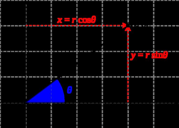
For example, consider a particle moving in a circular path. Its position is given by the displacement vector
For purposes of this example, set θ = t. The displacement (position) at any time t is then
This form shows the motion described by r(t) is in a circle of radius r because the magnitude of r(t) is given by
using the trigonometric identity sin2(t) + cos2(t) = 1 and where
With this form for the displacement, the velocity now is found. The time derivative of the displacement vector is the velocity vector. In general, the derivative of a vector is a vector made up of components each of which is the derivative of the corresponding component of the original vector. Thus, in this case, the velocity vector is:
Thus the velocity of the particle is nonzero even though the magnitude of the position (that is, the radius of the path) is constant. The velocity is directed perpendicular to the displacement, as can be established using the dot product:
Acceleration is then the time-derivative of velocity:
The acceleration is directed inward, toward the axis of rotation. It points opposite to the position vector and perpendicular to the velocity vector. This inward-directed acceleration is called centripetal acceleration.
Use in economics
In economics, many theoretical models of the evolution of various economic variables are constructed in continuous time and therefore employ time derivatives. See for example exogenous growth model and ch. 1-3. One situation involves a stock variable and its time derivative, a flow variable. Examples include:
Sometimes the time derivative of a flow variable can appear in a model:
And sometimes there appears a time derivative of a variable which, unlike the examples above, is not measured in units of currency: