Thermal resistance

Absolute thermal resistance

Absolute thermal resistance is the temperature difference across a structure when a unit of heat energy flows through it in unit time. It is the reciprocal of thermal conductance. The SI units of thermal resistance are kelvins per watt or the equivalent degrees Celsius per watt (the two are the same since the intervals are equal: Δ1 K = Δ1 °C).

The thermal resistance of materials is of great interest to electronic engineers because most electrical components generate heat and need to be cooled. Electronic components malfunction or fail if they overheat, and some parts routinely need measures taken in the design stage to prevent this.

Analogies

Electronic engineers are familiar with Ohm's law and so often use it as an analogy when doing calculations involving thermal resistance. Mechanical and Structural engineers are more familiar with Hooke's law and so often use it as an analogy when doing calculations involving thermal resistance.

Equivalent thermal circuits

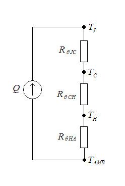
The heat flow can be modelled by analogy to an electrical circuit where heat flow is represented by current, temperatures are represented by voltages, heat sources are represented by constant current sources, absolute thermal resistances are represented by resistors and thermal capacitances by capacitors.

The diagram shows an equivalent thermal circuit for a semiconductor device with a heat sink.

Example calculation

Consider a component such as a silicon transistor that is bolted to the metal frame of a piece of equipment. The transistor's manufacturer will specify parameters in the datasheet called the absolute thermal resistance from junction to case (symbol: R θ J C ), and the maximum allowable temperature of the semiconductor junction (symbol: T J M A X ). The specification for the design should include a maximum temperature at which the circuit should function correctly. Finally, the designer should consider how the heat from the transistor will escape to the environment: this might be by convection into the air, with or without the aid of a heat sink, or by conduction through the printed circuit board. For simplicity, let us assume that the designer decides to bolt the transistor to a metal surface (or heat sink) that is guaranteed to be less than Δ T H S above the ambient temperature. Note: T_HS appears to be undefined.

Given all this information, the designer can construct a model of the heat flow from the semiconductor junction, where the heat is generated, to the outside world. In our example, the heat has to flow from the junction to the case of the transistor, then from the case to the metalwork. We do not need to consider where the heat goes after that, because we are told that the metalwork will conduct heat fast enough to keep the temperature less than Δ T H S above ambient: this is all we need to know.

Suppose the engineer wishes to know how much power he can put into the transistor before it overheats. The calculations are as follows.

Total absolute thermal resistance from junction to ambient = R θ J C + R θ B

where R θ B is the absolute thermal resistance of the bond between the transistor's case and the metalwork. This figure depends on the nature of the bond - for example, a thermal bonding pad or thermal transfer grease might be used to reduce the absolute thermal resistance.

Maximum temperature drop from junction to ambient = T J M A X − ( T A M B + Δ T H S ) .

We use the general principle that the temperature drop Δ T across a given absolute thermal resistance R θ with a given heat flow Q through it is:

Δ T = Q × R θ .

Substituting our own symbols into this formula gives:

T J M A X − ( T A M B + Δ T H S ) = Q M A X × ( R θ J C + R θ B + R θ H A ) ,

and, rearranging,

Q M A X = T J M A X − ( T A M B + Δ T H S ) R θ J C + R θ B + R θ H A

The designer now knows Q M A X , the maximum power that the transistor can be allowed to dissipate, so he can design the circuit to limit the temperature of the transistor to a safe level.

Let us substitute some sample numbers:

T J M A X = 125   ∘ C (typical for a silicon transistor) T A M B = 21   ∘ C (a typical specification for commercial equipment) R θ J C = 1.5   ∘ C / W (for a typical TO-220 package) R θ B = 0.1   ∘ C / W (a typical value for an elastomer heat-transfer pad for a TO-220 package) R θ H A = 4   ∘ C / W (a typical value for a heatsink for a TO-220 package)

The result is then:

Q = 125 − ( 21 ) 1.5 + 0.1 + 4 = 18.6   W

This means that the transistor can dissipate about 18 watts before it overheats. A cautious designer would operate the transistor at a lower power level to increase its reliability.

This method can be generalised to include any number of layers of heat-conducting materials, simply by adding together the absolute thermal resistances of the layers and the temperature drops across the layers.

Derived from Fourier's Law for heat conduction

From Fourier's Law for heat conduction, the following equation can be derived, and is valid as long as all of the parameters (x and k) are constant throughout the sample.

R θ = x A × k

where:

R θ is the absolute thermal resistance (across the length of the material) (K/W)

x is the length of the material (measured on a path parallel to the heat flow) (m)

k is the thermal conductivity of the material (W/(K·m))

A is the cross-sectional area (perpendicular to the path of heat flow) (m²)

Problems with electrical resistance analogy

A 2008 review paper written by Phillips researcher Clemens J. M. Lasance notes that: "Although there is an analogy between heat flow by conduction (Fourier’s law) and the flow of an electric current (Ohm’s law), the corresponding physical properties of thermal conductivity and electrical conductivity conspire to make the behavior of heat flow quite unlike the flow of electricity in normal situations. [...] Unfortunately, although the electrical and thermal differential equations are analogous, it is erroneous to conclude that there is any practical analogy between electrical and thermal resistance. This is because a material that is considered an insulator in electrical terms is about 20 orders of magnitude less conductive than a material that is considered a conductor, while, in thermal terms, the difference between an "insulator" and a "conductor" is only about three orders of magnitude. The entire range of thermal conductivity is then equivalent to the difference in electrical conductivity of high-doped and low-doped silicon."

Measurement standards

The junction-to-air thermal resistance can vary greatly depending on the ambient conditions. (A more sophisticated way of expressing the same fact is saying that junction-to-ambient thermal resistance is not Boundary-Condition Independent (BCI).) JEDEC has a standard (number JESD51-2) for measuring the junction-to-air thermal resistance of electronics packages under natural convection and another standard (number JESD51-6) for measurement under forced convection.

A JEDEC standard for measuring the junction-to-board thermal resistance (relevant for surface-mount technology) has been published as JESD51-8.

A JEDEC standard for measuring the junction-to-case thermal resistance (JESD51-14) is relatively newcomer, having been published in late 2010; it concerns only packages having a single heat flow and an exposed cooling surface.

Parallel thermal resistance

Similarly to electrical circuits, the total thermal resistance for steady state conditions can be calculated as follows.

The total thermal resistance

1 R t o t = 1 R B + 1 R C (1)

Simplifying the equation, we get

R t o t = R B R C R B + R C (2)

With terms for the thermal resistance for conduction, we get

R t , c o n d = L ( k b + k c ) A (3)

Resistance in series and parallel

It is often suitable to assume one-dimensional conditions, although the heat flow is multidimensional. Now, two different circuits may be used for this case. For case (a) (shown in picture), we presume isothermal surfaces for those normal to the x- direction, whereas for case (b) we presume adiabatic surfaces parallel to the x- direction. We may obtain different results for the total resistance R t o t and the actual corresponding values of the heat transfer are bracketed by q . When the multidimensional effects becomes more significant, these differences are increased with increasing | k f − k g | .

Radial Systems

Spherical and cylindrical systems may be treated as one-dimensional, due to the temperature gradients in the radial direction. The standard method can be used for analyzing radial systems under steady state conditions, starting with the appropriate form of the heat equation, or the alternative method, starting with the appropriate form of Fourier’s law. For a hollow cylinder in steady state conditions with no heat generation, the appropriate form of heat equation is

1 r d d r ( k r d T d r ) = 0 (4)

Where k is treated as a variable. Considering the appropriate form of Fourier’s law, the physical significance of treating k as a variable becomes evident when the rate at which energy is conducted across a cylindrical surface, this is represented as

q r = − k A d T d r = − k ( 2 π r L ) d T d r (5)

Where A = 2 π r L is the area that is normal to the direction of where the heat transfer occurs. Equation 1 implies that the quantity k r ( d T / d r ) is not dependent of the radius r , it follows from equation 5 that the heat transfer rate, q r is a constant in the radial direction.

In order to determine the temperature distribution in the cylinder, equation 4 can be solved applying the appropriate boundary conditions. With the assumption that k is constant

T ( r ) = C 1 l n r + C 2 (6)

Using the following boundary conditions, the constants C 1 and C 2 can be computed

T ( r 1 ) = T s , 1 and T ( r 2 ) = T s , 2

The general solution gives us

T s , 1 = C 1 l n r 1 + C 2 and T s , 1 = C 1 l n r 2 + C 2

Solving for C 1 and C 2 and substituting into the general solution, we obtain

T ( r ) = T s , 1 − T s , 2 l n ( r 2 / r 1 ) l n ( r r 2 ) + T s , 2 (7)

The logarithmic distribution of the temperature is sketched in the inset of the thumbnail figure. Assuming that the temperature distribution, equation 7, is used with Fourier’s law in equation 5, the heat transfer rate can be expressed in the following form

q r = 2 π L k ( T s , 1 − T s , 2 ) l n ( r 2 / r 1 )

Finally, for radial conduction in a cylindrical wall, the thermal resistance is of the form

R t , c o n d = l n ( r 2 / r 1 ) 2 π L k