Sudoku Codes

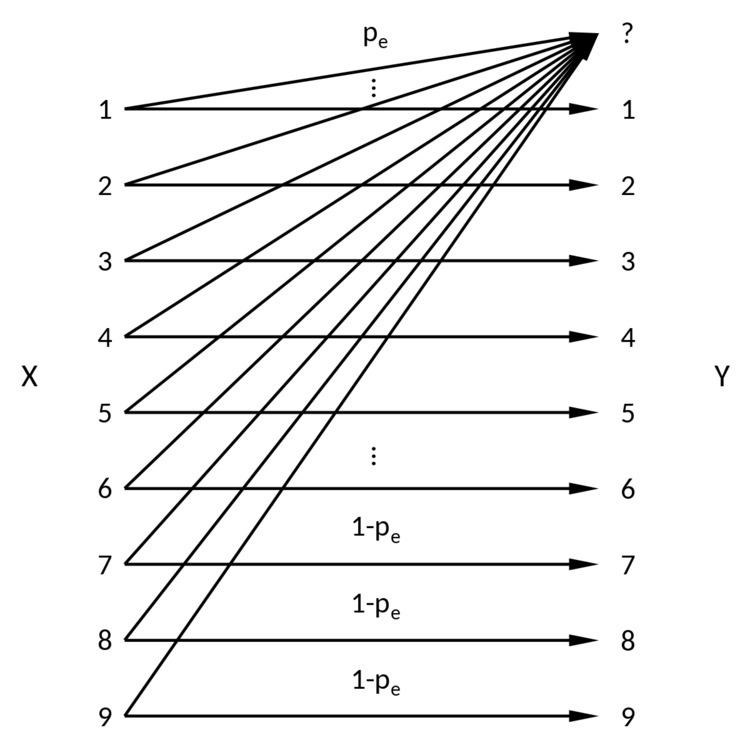
Erasure channel model

In the erasure channel model a symbol gets either transmitted correctly with probability 1 − p e or is erased with probability p e (see Figure \ref{fig:Sudoku3x3channel}). The channel introduces no errors, i.e. no channel input is changed to another symbol. The example in Figure \ref{fig:Sudoku3x3BSC} shows the transmission of a 3 × 3 Sudoku code. 5 of the 9 symbols got erased by the channel. The decoder is still able to reconstruct the message, i.e. the whole puzzle.

Note that the symbols sent over the channel are not binary. For a binary channel the symbols (e.g. integers { 1 , … , 9 } ) have to be mapped onto base 2. The binary erasure channel model however is not applicable because it erases only individual bits with some probability and not Sudoku symbols. If the symbols of the Sudoku are sent in packets the channel can be described as a packet erasure channel model.

Puzzle description

A sudoku is a N × N number-placement puzzle. It is filled in a way, that in each column, row and sub-grid N distinct symbols occur exactly once. Typical alphabet is the set of the integers { 1 , … , N } . The size of the sub-grids limit the size of SUDOKUs to N = n 2 with n ∈ N . Every solved sudoku and every sub-grid of it is a Latin square, meaning every symbol occurs exactly once in each row and column. At the starting point (in this case after the erasure channel) the puzzle is only partially complete but has only one unique solution.

For channel codes also other varieties of sudokus are conceivable. Diagonal regions instead of square sub-grids can be used for performance investigations. The diagonal sudoku has the advantage, that its size can be chosen more freely. Due to the sub-grid structure normal sudokus can only be of size n², diagonal sudokus have valid solutions for all odd N .

Sudoku codes are non-linear. In a linear code any linear combination of codewords give a new valid codeword, this does not hold for sudoku codes. The symbols of a sudoku are from a finite alphabet (e.g. integers { 1 , … , 9 } ). The constraints of Sudoku codes are non-linear: all symbols within a constraint (row, line, sub-grid) must be different from any other symbol within this constraint. Hence there is no all-zero codeword in Sudoku codes.

Sudoku codes can be represented by probabilistic graphical model in which they take the form of a low-density parity-check code.

Decoding with belief propagation

There are several possible decoding methods for sudoku codes. Some algorithms are very specific developments for Sudoku codes. Several methods are described in sudoku solving algorithms. Another efficient method is with dancing links.

Decoding methods like belief propagation are also used for low-density parity-check codes are of special interest. Performance analysis of these methods on sudoku codes can help to understand decoding problems for low-density parity-check codes better.

By modeling sudoku codes as a probabilistic graphical model belief propagation can be used for Sudoku codes. Belief propagation on the tanner graph or factor graph to decode Sudoku codes is discussed in by Sayir. and Moon This method is originally designed for low-density parity-check codes. Due to its generality belief propagation works not only with the classical 9 × 9 Sudoku but with a variety of those. LDPC decoding is a common use-case for belief propagation, with slight modifications this approach can be used for solving Sudoku codes.

The constraint satisfaction using a tanner graph is shown in the figure on the right. S n denotes the entries of the sudoku in row-scan order. C m denotes the constraint functions: m = 1 , . . . , 9 associated with rows, m = 10 , . . . , 18 associated with columns and m = 19 , . . . , 27 associated with the 3 × 3 sub-grids of the Sudoku. C m is defined as

C m ( s 1 , s 2 , . . . . . , s 9 ) = { 1 , if  s 1 , s 2 , . . . , s 9  are distinct 0 , otherwise.

Every cell S n is connected to 3 constraints: the row, column and sub-grid constraints. A specification of the general approach for belief propagation is suggested by Sayir: The initial probability of a received symbol is either 1 to the observed symbol and 0 to all others or uniform distributed on the whole alphabet if the symbol is erased. For the belief propagation algorithm it is sufficient to transmit only a subset of possibilities instead of distributions, since the distribution is always uniform over the subset. The candidates for the erased symbols narrow down to a subset of the alphabet as symbols get excluded due to constraints. All values that are used by another cell in the constraint, and pairs that are shared among two other cells and so on are eliminated. Sudoku players use this method of logic excluding to solve most sudoku puzzles.

Encoding

The aim of error-correcting codes is to encode data in a way such that it is more resilient to errors in the transmission process. The encoder has to map data U to a valid sudoku grid from which the codeword X can we taken e.g. in row-scan order.

shows the necessary steps.

A standard 9 × 9 sudoku has about 72.5 bits of information as calculated in the next section. Information after Shannon is the degree of randomness in a set of data. An ideal coin toss for example has an information of I = log 2 ⁡ 2 = 1 bit. To represent the outcome of 72 coin tosses 72 bits are necessary. One Sudoku contains therewith about the same information as 72 coin tosses or a sequence of 72 bits. A sequence of 81 random symbols { 1 , … , 9 } has I = 81 log 2 ⁡ 9 ≈ 256.8 bits of information. One Sudoku code can be seen as 72.5 bits of information and 184.3 bits redundancy. Theoretically a string of 72 bits can be mapped to one sudoku that is sent over the channel as a string of 81 symbols. However, there is no linear function that maps a string to a sudoku code.

A suggested encoding approach by Sayir is as follows:

For a 4 × 4 sudoku the first entry can be filled with a source of cardinality 4. In this example this a 1. For the rest of this row, column and 2 × 2 sub-grid this number is excluded from the possibilities in the belief propagation decoder. For the second cell only the numbers 2,3,4 are valid. The source has to be transformed into a uniform distribution between three possibilities and mapped to the valid numbers and so on, until the grid is filled.

Performance of sudoku codes

The calculation of the rate of sudoku codes is not trivial. An example rate calculation of a 4 × 4 sudoku is shown above. Filling line by line from the top left corner only the first entry has maximum information of log 2 ⁡ 4 = 2 bits. Every next entry cannot be any of the numbers used before, so the information reduces to log 2 ⁡ 3 , log 2 ⁡ 2 and 0 for the following entries, as they have to be of the remaining left numbers. In the second lines the information is additionally reduced by the area rule: cell 5 in row-scan order can only be a 3 or 4 as the numbers 1 and 2 are already used in the sub-grid. The last row contains no information at all. Adding all information up one gets log ⁡ ( 4 ∗ 3 ∗ 2 5 ) ≈ 8.58 bits. The rate in this example is

The exact number of possible Sudoku grids according to Mathematics of Sudoku is 6 , 670 , 903 , 752 , 021 , 072 , 936 , 960 . With the total information of

the average rate of a standard Sudoku is

The average number of possible entries for a cell is 6.67 ∗ 10 21 81 ≈ 1.86 or log 2 ⁡ 1.86 ≈ 0.90 bits of information per Sudoku cell. Note that the rate may vary between codewords.

The minimum number of given entries that render a unique solution was proven to be 17. In the worst case only four missing entries can lead to ambiguous solutions. For an erasure channel it is very unlikely that 17 successful transmissions are enough to reproduce the puzzle. There are only about 50,000 known solutions with 17 given entries.

Density evolution

Density evolution is a capacity analysis algorithm originally developed for low-density parity-check codes on belief propagation decoding. Density evolution can also be applied to Sudoku-type constraints. One important simplification used in density evolution on LDPC codes is the sufficiency to analyze only the all-one codeword. With the Sudoku constraints however, this is not a valid codeword. Unlike for linear codes the weight-distance equivalence property does not hold for non-linear codes. Therewith it is necessary to compute density evolution recursions for every possible Sudoku puzzle to get precise performance analysis.

A proposed simplification is to analyze the probability distribution of the cardinalities of messages instead of the probability distribution of the message. Density evolution is calculated on the entry nodes and the constraint nodes (compare Tanner graph above). On the entry nodes one analyzes the cardinalities of the constraints. If for example the constraints have the cardinalities ( 1 , 1 ) then the entry can only be of one symbol. If the constraints have cardinalities ( 2 , 2 ) then both constraints allow two different symbols. For both constraints the correct symbol is contained for sure, lets assume the correct symbol is 1 . The other symbol can be equal or different for the constraints. If the symbols are different then the correct symbol is determined. If the second symbol is equal, lets assume 2 the output symbols are of cardinality 2 i.e. the symbols { 1 , 2 } . Depending on the alphabet size ( q ) the probability for the unique output for the input cardinalities ( 2 , 2 ) is

and for output of cardinality 2

For a standard 9 × 9 Sudoku this results in a probability of 7 / 8 for a unique solution. An analog calculation is done for all cardinality combinations. In the end the distribution of output cardinalities are summed up from the results. Note that the order of the input cardinality is interchangeable. The calculation of non-decreasing constraint combinations is therewith sufficient.

For constraint nodes the procedure is somewhat similar and described in the following example based on a 4 × 4 standard Sudoku. Inputs to the constraint nodes are the possible symbols of the connected entry nodes. Cardinality 1 means that the symbol of the source node is already determined. Again a non-decreasing analysis is sufficient. Lets assume the true output value is 4 and the inputs have cardinalities ( 1 , 1 , 2 ) with the true symbols 1-2-3. The messages with cardinality 1 are { 1 } and { 2 } . The message of cardinality 2 might be { 1 , 3 } , { 2 , 3 } or { 3 , 4 } as the true symbol 3 must be contained. In two of three cases the output is the correct symbol 4 with cardinality 1: { 1 } , { 2 } , { 1 , 3 } and { 1 } , { 2 } , { 2 , 3 } . In one of three case the output cardinality is 2: { 1 } , { 2 } , { 3 , 4 } . The output symbols in this case are { 3 , 4 } . The final output cardinality distribution can be expressed by summing over all possible input combinations. For a 4 × 4 standard Sudoku these are 64 combinations that can be grouped to 20 non-decreasing ones.

If the cardinality converges to 1 the decoding is error-free. To find the threshold the erasure probability must be increased until the decoding error remains positive for any number of iterations. With the method of Sayir density evolution recursions can be used to calculate thresholds also for Sudoku codes up to an alphabet size q = 8 .