Stochastic matrix

Definition and properties

A stochastic matrix describes a Markov chain X t over a finite state space S with cardinality S .

If the probability of moving from i to j in one time step is P r ( j | i ) = P i , j , the stochastic matrix P is given by using P i , j as the i t h row and j t h column element, e.g.,

Since the total of transition probability from a state i to all other states must be 1, this matrix is a right stochastic matrix, so that

The product of two right stochastic matrices is also right stochastic. In particular, the k -th power P k of a right stochastic matrix P is also right stochastic. The probability of transitioning from i to j in two steps is then given by the ( i , j ) t h element of the square of P :

In general the probability transition of going from any state to another state in a finite Markov chain given by the matrix P in k steps is given by P k .

An initial distribution is given as a row vector.

A stationary probability vector π is defined as a distribution, written as a row vector, that does not change under application of the transition matrix; that is, it is defined as a probability distribution on the set { 1 , . . . , n } which is also a row eigenvector of the probability matrix, associated with eigenvalue 1:

The right spectral radius of every right stochastic matrix is clearly at most 1. Additionally, every right stochastic matrix has an obvious column eigenvector associated to the eigenvalue 1: The vector 1 , whose coordinates are all equal to 1. As left and right eigenvalues of a square matrix are the same, every stochastic matrix has, at least, a row eigenvector associated to the eigenvalue 1 and the largest absolute value of all its eigenvalues is also 1. Finally, the Brouwer Fixed Point Theorem (applied to the compact convex set of all probability distributions of the finite set { 1 , . . . , n } ) implies that there is some left eigenvector which is also a stationary probability vector.

On the other hand, the Perron–Frobenius theorem also ensures that every irreducible stochastic matrix has such a stationary vector, and that the largest absolute value of an eigenvalue is always 1. However, this theorem cannot be applied directly to such matrices because they need not be irreducible.

In general, there may be several such vectors. However, for a matrix with strictly positive entries (or, more generally, for an irreducible aperiodic stochastic matrix), this vector is unique and can be computed by observing that for any i we have the following limit,

where π j is the j t h element of the row vector π . Among other things, this says that the long-term probability of being in a state j is independent of the initial state i . That both of these computations give the same stationary vector is a form of an ergodic theorem, which is generally true in a wide variety of dissipative dynamical systems: the system evolves, over time, to a stationary state.

Intuitively, a stochastic matrix represents a Markov chain; the application of the stochastic matrix to a probability distribution redistributes the probability mass of the original distribution while preserving its total mass. If this process is applied repeatedly, the distribution converges to a stationary distribution for the Markov chain.

Example: the cat and mouse

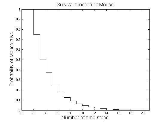
Suppose you have a timer and a row of five adjacent boxes, with a cat in the first box and a mouse in the fifth box at time zero. The cat and the mouse both jump to a random adjacent box when the timer advances. E.g. if the cat is in the second box and the mouse in the fourth one, the probability is one fourth that the cat will be in the first box and the mouse in the fifth after the timer advances. If the cat is in the first box and the mouse in the fifth one, the probability is one that the cat will be in box two and the mouse will be in box four after the timer advances. The cat eats the mouse if both end up in the same box, at which time the game ends. The random variable K gives the number of time steps the mouse stays in the game.

The Markov chain that represents this game contains the following five states specified by the combination of positions (cat,mouse). Note that while a naive enumeration of states would list 25 states, many are impossible either because the mouse can never have a lower index than the cat (as that would mean the mouse occupied the cat's box and survived to move past it), or because the sum of the two indices will always have even parity. In addition, the 3 possible states that lead to the mouse's death are combined into one:

We use a stochastic matrix to represent the transition probabilities of this system (rows and columns in this matrix are indexed by the possible states listed above, with the pre-transition state as the row and post-transition state as the column).

Long-term averages

No matter what the initial state, the cat will eventually catch the mouse (with probability 1) and a stationary state π = (0,0,0,0,1) is approached as a limit. To compute the long-term average or expected value of a stochastic variable Y, for each state S_j and time t_k there is a contribution of Y_j,k·P(S=S_j,t=t_k). Survival can be treated as a binary variable with Y=1 for a surviving state and Y=0 for the terminated state. The states with Y=0 do not contribute to the long-term average.

Phase-type representation

As State 5 is an absorbing state, the distribution of time to absorption is discrete phase-type distributed. Suppose the system starts in state 2, represented by the vector [ 0 , 1 , 0 , 0 , 0 ] . The states where the mouse has perished don't contribute to the survival average so state five can be ignored. The initial state and transition matrix can be reduced to,

and,

where I is the identity matrix, and 1 represents a column matrix of all ones that acts as a sum over states.

Since each state is occupied for one step of time the expected time of the mouse's survival is just the sum of the probability of occupation over all surviving states and steps in time,

Higher order moments are given by