Stencil code

Definition

Stencil codes perform a sequence of sweeps (called timesteps) through a given array. Generally this is a 2- or 3-dimensional regular grid. The elements of the arrays are often referred to as cells. In each timestep, the stencil code updates all array elements. Using neighboring array elements in a fixed pattern (called the stencil), each cell's new value is computed. In most cases boundary values are left unchanged, but in some cases (e.g. LBM codes) those need to be adjusted during the computation as well. Since the stencil is the same for each element, the pattern of data accesses is repeated.

More formally, we may define stencil codes as a 5-tuple ( I , S , S 0 , s , T ) with the following meaning:

Since I is a k-dimensional integer interval, the array will always have the topology of a finite regular grid. The array is also called simulation space and individual cells are identified by their index c ∈ I . The stencil is an ordered set of l relative coordinates. We can now obtain for each cell c the tuple of its neighbors indices I c

Their states are given by mapping the tuple I c to the corresponding tuple of states N i ( c ) , where N i : I → S l is defined as follows:

This is all we need to define the system's state for the following time steps S i + 1 : Z k → S with i ∈ N :

Note that S i is defined on Z k and not just on I since the boundary conditions need to be set, too. Sometimes the elements of I c may be defined by a vector addition modulo the simulation space's dimension to realize toroidal topologies:

This may be useful for implementing periodic boundary conditions, which simplifies certain physical models.

Example: 2D Jacobi iteration

To illustrate the formal definition, we'll have a look at how a two dimensional Jacobi iteration can be defined. The update function computes the arithmetic mean of a cell's four neighbors. In this case we set off with an initial solution of 0. The left and right boundary are fixed at 1, while the upper and lower boundaries are set to 0. After a sufficient number of iterations, the system converges against a saddle-shape.

Stencils

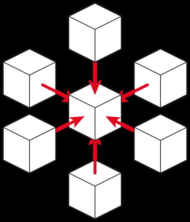
The shape of the neighborhood used during the updates depends on the application itself. The most common stencils are the 2D or 3D versions of the von Neumann neighborhood and Moore neighborhood. The example above uses a 2D von Neumann stencil while LBM codes generally use its 3D variant. Conway's Game of Life uses the 2D Moore neighborhood. That said, other stencils such as a 25-point stencil for seismic wave propagation can be found, too.

Implementation issues

Many simulation codes may be formulated naturally as stencil codes. Since computing time and memory consumption grow linearly with the number of array elements, parallel implementations of stencil codes are of paramount importance to research. This is challenging since the computations are tightly coupled (because of the cell updates depending on neighboring cells) and most stencil codes are memory bound (i.e. the ratio of memory accesses to calculations is high). Virtually all current parallel architectures have been explored for executing stencil codes efficiently; at the moment GPGPUs have proven to be most efficient.

Libraries

Due to both, the importance of stencil codes to computer simulations and their high computational requirements, there are a number of efforts which aim at creating reusable libraries to support scientists in implementing new stencil codes. The libraries are mostly concerned with the parallelization, but may also tackle other challenges, such as IO, steering and checkpointing. They may be classified by their API.

Patch-based libraries

This is a traditional design. The library manages a set of n-dimensional scalar arrays, which the user code may access to perform updates. The library handles the synchronization of the boundaries (dubbed ghost zone or halo). The advantage of this interface is that the user code may loop over the arrays, which makes it easy to integrate legacy codes . The disadvantage is that the library can not handle cache blocking (as this has to be done within the loops) or wrapping of the code for accelerators (e.g. via CUDA or OpenCL). Notable implementations include Cactus, a physics problem solving environment, and waLBerla.

Cell-based libraries

These libraries move the interface to updating single simulation cells: only the current cell and its neighbors are exposed to the user code, e.g. via getter/setter methods. The advantage of this approach is that the library can control tightly which cells are updated in which order, which is useful not only to implement cache blocking, but also to run the same code on multi-cores and GPUs. This approach requires the user to recompile the source code together with the library. Otherwise a function call for every cell update would be required, which would seriously impair performance. This is only feasible with techniques such as class templates or metaprogramming, which is also the reason why this design is only found in newer libraries. Examples are Physis and LibGeoDecomp.