
 | ||
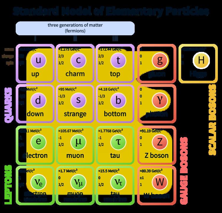
This article describes the mathematics of the Standard Model of particle physics, a gauge quantum field theory containing the internal symmetries of the unitary product group SU(3) × SU(2) × U(1). The theory is commonly viewed as containing the fundamental set of particles – the leptons, quarks, gauge bosons and the Higgs particle.
Contents
- Quantum field theory
- The role of the quantum fields
- Vectors scalars and spinors
- Alternative presentations of the fields
- Fermions
- A chiral theory
- Mass and interaction eigenstates
- Positive and negative energies
- Bosons
- Perturbative QFT and the interaction picture
- Free fields
- Interaction terms and the path integral approach
- Lagrangian formalism
- Kinetic terms
- Fermion fields
- Gauge fields
- Coupling terms
- Electroweak sector
- Quantum chromodynamics sector
- Mass terms
- The Higgs mechanism
- Neutrino masses
- Detailed information
- Field content in detail
- Fermion content
- Free parameters
- Additional symmetries of the Standard Model
- The U1 symmetry
- The charged and neutral current couplings and Fermi theory
- References
The Standard Model is renormalizable and mathematically self-consistent, however despite having huge and continued successes in providing experimental predictions it does leave some unexplained phenomena. In particular, although the physics of special relativity is incorporated, general relativity is not, and the Standard Model will fail at energies or distances where the graviton is expected to emerge. Therefore, in a modern field theory context, it is seen as an effective field theory.
This article requires some background in physics and mathematics, but is designed as both an introduction and a reference.
Quantum field theory
The standard model is a quantum field theory, meaning its fundamental objects are quantum fields which are defined at all points in spacetime. These fields are
That these are quantum rather than classical fields has the mathematical consequence that they are operator-valued. In particular, values of the fields generally do not commute. As operators, they act upon the quantum state (ket vector).
The dynamics of the quantum state and the fundamental fields are determined by the Lagrangian density
The standard model is furthermore a gauge theory, which means there are degrees of freedom in the mathematical formalism which do not correspond to changes in the physical state. The gauge group of the standard model is SU(3) × SU(2) × U(1), where U(1) acts on B and φ, SU(2) acts on W and φ, and SU(3) acts on G. The fermion field ψ also transforms under these symmetries, although all of them leave some parts of it unchanged.
The role of the quantum fields
In classical mechanics, the state of a system can usually be captured by a small set of variables, and the dynamics of the system is thus determined by the time evolution of these variables. In classical field theory, the field is part of the state of the system, so in order to describe it completely one effectively introduces separate variables for every point in spacetime (even though there are many restrictions on how the values of the field "variables" may vary from point to point, for example in the form of field equations involving partial derivatives of the fields).
In quantum mechanics, the classical variables are turned into operators, but these do not capture the state of the system, which is instead encoded into a wavefunction ψ or more abstract ket vector. If ψ is an eigenstate with respect to an operator P, then Pψ = λψ for the corresponding eigenvalue λ, and hence letting an operator P act on ψ is analogous to multiplying ψ by the value of the classical variable to which P corresponds. By extension, a classical formula where all variables have been replaced by the corresponding operators will behave like an operator which, when it acts upon the state of the system, multiplies it by the analogue of the quantity that the classical formula would compute. The formula as such does however not contain any information about the state of the system; it would evaluate to the same operator regardless of what state the system is in.
Quantum fields relate to quantum mechanics as classical fields do to classical mechanics, i.e., there is a separate operator for every point in spacetime, and these operators do not carry any information about the state of the system; they are merely used to exhibit some aspect of the state, at the point to which they belong. In particular, the quantum fields are not wavefunctions, even though the equations which govern their time evolution may be deceptively similar to those of the corresponding wavefunction in a semiclassical formulation. There is no variation in strength of the fields between different points in spacetime; the variation that happens is rather one of phase factors.
Vectors, scalars, and spinors
Mathematically it may look as though all of the fields are vector-valued (in addition to being operator-valued), since they all have several components, can be multiplied by matrices, etc., but physicists assign a more specific physical meaning to the word: a vector is something which transforms like a four-vector under Lorentz transformations, and a scalar is something which is invariant under Lorentz transformations. The B, Wj, and Ga fields are all vectors in this sense, so the corresponding particles are said to be vector bosons. The Higgs field φ is a scalar.
The fermion field ψ does transform under Lorentz transformations, but not like a vector should; rotations will only turn it by half the angle a proper vector should. Therefore, these constitute a third kind of quantity, which is known as a spinor.
It is common to make use of abstract index notation for the vector fields, in which case the vector fields all come with a Lorentzian index μ, like so:
Alternative presentations of the fields
As is common in quantum theory, there is more than one way to look at things. At first the basic fields given above may not seem to correspond well with the "fundamental particles" in the chart above, but there are several alternative presentations which, in particular contexts, may be more appropriate than those that are given above.
Fermions
Rather than having one fermion field ψ, it can be split up into separate components for each type of particle. This mirrors the historical evolution of quantum field theory, since the electron component ψe (describing the electron and its antiparticle the positron) is then the original ψ field of quantum electrodynamics, which was later accompanied by ψμ and ψτ fields for the muon and tauon respectively (and their antiparticles). Electroweak theory added
An important definition is the barred fermion field
A chiral theory
An independent decomposition of ψ is that into chirality components:
"Left" chirality:where
In particular, under weak isospin SU(2) transformations the left-handed particles are weak-isospin doublets, whereas the right-handed are singlets – i.e. the weak isospin of ψR is zero. Put more simply, the weak interaction could rotate e.g. a left-handed electron into a left-handed neutrino (with emission of a W−), but could not do so with the same right-handed particles. As an aside, the right-handed neutrino originally did not exist in the standard model – but the discovery of neutrino oscillation implies that neutrinos must have mass, and since chirality can change during the propagation of a massive particle, right-handed neutrinos must exist in reality. This does not however change the (experimentally-proven) chiral nature of the weak interaction.
Furthermore, U(1) acts differently on
Mass and interaction eigenstates
A distinction can thus be made between, for example, the mass and interaction eigenstates of the neutrino. The former is the state which propagates in free space, whereas the latter is the different state that participates in interactions. Which is the "fundamental" particle? For the neutrino, it is conventional to define the "flavour" (
ν
e,
ν
μ, or
ν
τ) by the interaction eigenstate, whereas for the quarks we define the flavour (up, down, etc.) by the mass state. We can switch between these states using the CKM matrix for the quarks, or the PMNS matrix for the neutrinos (the charged leptons on the other hand are eigenstates of both mass and flavour).
As an aside, if a complex phase term exists within either of these matrices, it will give rise to direct CP violation, which could explain the dominance of matter over antimatter in our current universe. This has been proven for the CKM matrix, and is expected for the PMNS matrix.
Positive and negative energies
Finally, the quantum fields are sometimes decomposed into "positive" and "negative" energy parts: ψ = ψ+ + ψ−. This is not so common when a quantum field theory has been set up, but often features prominently in the process of quantizing a field theory.
Bosons
Due to the Higgs mechanism, the electroweak boson fields
The massive neutral (Z) boson:
The massless neutral boson:
The massive charged W bosons:
where θW is the Weinberg angle.
The A field is the photon, which corresponds classically to the well-known electromagnetic four-potential – i.e. the electric and magnetic fields. The Z field actually contributes in every process the photon does, but due to its large mass, the contribution is usually negligible.
Perturbative QFT and the interaction picture
Much of the qualitative descriptions of the standard model in terms of "particles" and "forces" comes from the perturbative quantum field theory view of the model. In this, the Langrangian is decomposed as
In the more common Schrödinger picture, even the states of free particles change over time: typically the phase changes at a rate which depends on their energy. In the alternative Heisenberg picture, state vectors are kept constant, at the price of having the operators (in particular the observables) be time-dependent. The interaction picture constitutes an intermediate between the two, where some time dependence is placed in the operators (the quantum fields) and some in the state vector. In QFT, the former is called the free field part of the model, and the latter is called the interaction part. The free field model can be solved exactly, and then the solutions to the full model can be expressed as perturbations of the free field solutions, for example using the Dyson series.
It should be observed that the decomposition into free fields and interactions is in principle arbitrary. For example, renormalization in QED modifies the mass of the free field electron to match that of a physical electron (with an electromagnetic field), and will in doing so add a term to the free field Lagrangian which must be cancelled by a counterterm in the interaction Lagrangian, that then shows up as a two-line vertex in the Feynman diagrams. This is also how the Higgs field is thought to give particles mass: the part of the interaction term which corresponds to the (nonzero) vacuum expectation value of the Higgs field is moved from the interaction to the free field Lagrangian, where it looks just like a mass term having nothing to do with Higgs.
Free fields
Under the usual free/interaction decomposition, which is suitable for low energies, the free fields obey the following equations:
These equations can be solved exactly. One usually does so by considering first solutions that are periodic with some period L along each spatial axis; later taking the limit: L → ∞ will lift this periodicity restriction.
In the periodic case, the solution for a field F (any of the above) can be expressed as a Fourier series of the form
where:
In the limit L → ∞, the sum would turn into an integral with help from the V hidden inside β. The numeric value of β also depends on the normalization chosen for
Technically,
An important step in preparation for calculating in perturbative quantum field theory is to separate the "operator" factors a and b above from their corresponding vector or spinor factors u and v. The vertices of Feynman graphs come from the way that u and v from different factors in the interaction Lagrangian fit together, whereas the edges come from the way that the as and bs must be moved around in order to put terms in the Dyson series on normal form.
Interaction terms and the path integral approach
The Lagrangian can also be derived without using creation and annihilation operators (the "canonical" formalism), by using a "path integral" approach, pioneered by Feynman building on the earlier work of Dirac. See e.g. Path integral formulation on Wikipedia or A. Zee's QFT in a nutshell. This is one possible way that the Feynman diagrams, which are pictorial representations of interaction terms, can be derived relatively easily. A quick derivation is indeed presented at the article on Feynman diagrams.
Lagrangian formalism
We can now give some more detail about the aforementioned free and interaction terms appearing in the Standard Model Lagrangian density. Any such term must be both gauge and reference-frame invariant, otherwise the laws of physics would depend on an arbitrary choice or the frame of an observer. Therefore, the global Poincaré symmetry, consisting of translational symmetry, rotational symmetry and the inertial reference frame invariance central to the theory of special relativity must apply. The local SU(3) × SU(2) × U(1) gauge symmetry is the internal symmetry. The three factors of the gauge symmetry together give rise to the three fundamental interactions, after some appropriate relations have been defined, as we shall see.
A complete formulation of the Standard Model Lagrangian with all the terms written together can be found e.g. here.
Kinetic terms
A free particle can be represented by a mass term, and a kinetic term which relates to the "motion" of the fields.
Fermion fields
The kinetic term for a Dirac fermion is
where the notations are carried from earlier in the article. ψ can represent any, or all, Dirac fermions in the standard model. Generally, as below, this term is included within the couplings (creating an overall "dynamical" term).
Gauge fields
For the spin-1 fields, first define the field strength tensor
for a given gauge field (here we use A), with gauge coupling constant g. The quantity f abc is the structure constant of the particular gauge group, defined by the commutator
where ti are the generators of the group. In an Abelian (commutative) group (such as the U(1) we use here), since the generators ta all commute with each other, the structure constants vanish. Of course, this is not the case in general – the standard model includes the non-Abelian SU(2) and SU(3) groups (such groups lead to what is called a Yang–Mills gauge theory).
We need to introduce three gauge fields corresponding to each of the subgroups SU(3) × SU(2) × U(1).
The kinetic term can now be written simply as
where the traces are over the SU(2) and SU(3) indices hidden in W and G respectively. The two-index objects are the field strengths derived from W and G the vector fields. There are also two extra hidden parameters: the theta angles for SU(2) and SU(3).
Coupling terms
The next step is to "couple" the gauge fields to the fermions, allowing for interactions.
Electroweak sector
The electroweak sector interacts with the symmetry group U(1) × SU(2)L, where the subscript L indicates coupling only to left-handed fermions.
Where Bμ is the U(1) gauge field; YW is the weak hypercharge (the generator of the U(1) group); Wμ is the three-component SU(2) gauge field; and the components of τ are the Pauli matrices (infinitesimal generators of the SU(2) group) whose eigenvalues give the weak isospin. Note that we have to redefine a new U(1) symmetry of weak hypercharge, different from QED, in order to achieve the unification with the weak force. The electric charge Q, third component of weak isospin T3 (also called Tz, I3 or Iz) and weak hypercharge YW are related by
or by the alternate convention Q = T3 + YW. The first convention (used in this article) is equivalent to the earlier Gell-Mann–Nishijima formula. We can then define the conserved current for weak isospin as
and for weak hypercharge as
where
To explain in a simpler way, we can see the effect of the electroweak interaction by picking out terms from the Lagrangian. We see that the SU(2) symmetry acts on each (left-handed) fermion doublet contained in ψ, for example
where the particles are understood to be left-handed, and where
This is an interaction corresponding to a "rotation in weak isospin space" or in other words, a transformation between eL and νeL via emission of a W− boson. The U(1) symmetry, on the other hand, is similar to electromagnetism, but acts on all "weak hypercharged" fermions (both left and right handed) via the neutral Z0, as well as the charged fermions via the photon.
Quantum chromodynamics sector
The quantum chromodynamics (QCD) sector defines the interactions between quarks and gluons, with SU(3) symmetry, generated by Ta. Since leptons do not interact with gluons, they are not affected by this sector. The Dirac Lagrangian of the quarks coupled to the gluon fields is given by
where D and U are the Dirac spinors associated with up- and down-type quarks, and other notations are continued from the previous section.
Mass terms
The mass term arising from the Dirac Lagrangian (for any fermion ψ) is
i.e. contribution from
The Higgs mechanism
The solution to both these problems comes from the Higgs mechanism, which involves scalar fields (the number of which depend on the exact form of Higgs mechanism) which (to give the briefest possible description) are "absorbed" by the massive bosons as degrees of freedom, and which couple to the fermions via Yukawa coupling to create what looks like mass terms.
In the Standard Model, the Higgs field is a complex scalar of the group SU(2)L:
where the superscripts + and 0 indicate the electric charge (Q) of the components. The weak hypercharge (YW) of both components is 1.
The Higgs part of the Lagrangian is
where λ > 0 and μ2 > 0, so that the mechanism of spontaneous symmetry breaking can be used. There is a parameter here, at first hidden within the shape of the potential, that is very important. In a unitarity gauge one can set φ+ = 0 and make φ0 real. Then
The Yukawa interaction terms are
where Gu,d are 3 × 3 matrices of Yukawa couplings, with the ij term giving the coupling of the generations i and j.
Neutrino masses
As previously mentioned, evidence shows neutrinos must have mass. But within the standard model, the right-handed neutrino does not exist, so even with a Yukawa coupling neutrinos remain massless. An obvious solution is to simply add a right-handed neutrino νR resulting in a Dirac mass term as usual. This field however must be a sterile neutrino, since being right-handed it experimentally belongs to an isospin singlet (T3 = 0) and also has charge Q = 0, implying YW = 0 (see above) i.e. it does not even participate in the weak interaction. Current experimental status is that evidence for observation of sterile neutrinos is not convincing.
Another possibility to consider is that the neutrino satisfies the Majorana equation, which at first seems possible due to its zero electric charge. In this case the mass term is
where C denotes a charge conjugated (i.e. anti-) particle, and the terms are consistently all left (or all right) chirality (note that a left-chirality projection of an antiparticle is a right-handed field; care must be taken here due to different notations sometimes used). Here we are essentially flipping between LH neutrinos and RH anti-neutrinos (it is furthermore possible but not necessary that neutrinos are their own antiparticle, so these particles are the same). However, for the left-chirality neutrinos, this term changes weak hypercharge by 2 units - not possible with the standard Higgs interaction, requiring the Higgs field to be extended to include an extra triplet with weak hypercharge 2 - whereas for right-chirality neutrinos, no Higgs extensions are necessary. For both left and right chirality cases, Majorana terms violate lepton number, but possibly at a level beyond the current sensitivity of experiments to detect such violations.
It is possible to include both Dirac and Majorana mass terms in the same theory, which (in contrast to the Dirac-mass-only approach) can provide a "natural" explanation for the smallness of the observed neutrino masses, by linking the RH neutrinos to yet-unknown physics around the GUT scale (see seesaw mechanism).
Since in any case new fields must be postulated to explain the experimental results, neutrinos are an obvious gateway to searching physics beyond the Standard Model.
Detailed information
This section provides more detail on some aspects, and some reference material.
Field content in detail
The Standard Model has the following fields. These describe one generation of leptons and quarks, and there are three generations, so there are three copies of each field. By CPT symmetry, there is a set of right-handed fermions with the opposite quantum numbers. The column "representation" indicates under which representations of the gauge groups that each field transforms, in the order (SU(3), SU(2), U(1)). Symbols used are common but not universal; superscript C denotes an antiparticle; and for the U(1) group, the value of the weak hypercharge is listed. Note that there are twice as many left-handed lepton field components as left-handed antilepton field components in each generation, but an equal number of left-handed quark and antiquark fields.
Fermion content
This table is based in part on data gathered by the Particle Data Group.
Free parameters
Upon writing the most general Lagrangian without neutrinos, one finds that the dynamics depend on 19 parameters, whose numerical values are established by experiment. With neutrinos 7 more parameters are needed, 3 masses and 4 PMNS matrix parameters, for a total of 26 parameters. The neutrino parameter values are still uncertain. The 19 certain parameters are summarized here.
The choice of free parameters is somewhat arbitrary. In the table above, gauge couplings are listed as free parameters, therefore with this choice Weinberg angle is not a free parameter - it is defined as
Instead of fermion masses, dimensionless Yukawa couplings can be chosen as free parameters. For example, electron mass depends on the Yukawa coupling of electron to Higgs field, and its value is
Instead of the Higgs mass, the Higgs self-coupling strength λ ~ ⅛ can be chosen as a free parameter.
Additional symmetries of the Standard Model
From the theoretical point of view, the Standard Model exhibits four additional global symmetries, not postulated at the outset of its construction, collectively denoted accidental symmetries, which are continuous U(1) global symmetries. The transformations leaving the Lagrangian invariant are:
The first transformation rule is shorthand meaning that all quark fields for all generations must be rotated by an identical phase simultaneously. The fields ML, TL and
By Noether's theorem, each symmetry above has an associated conservation law: the conservation of baryon number, electron number, muon number, and tau number. Each quark is assigned a baryon number of
Similarly, each electron and its associated neutrino is assigned an electron number of +1, while the anti-electron and the associated anti-neutrino carry a −1 electron number. Similarly, the muons and their neutrinos are assigned a muon number of +1 and the tau leptons are assigned a tau lepton number of +1. The Standard Model predicts that each of these three numbers should be conserved separately in a manner similar to the way baryon number is conserved. These numbers are collectively known as lepton family numbers (LF).
In addition to the accidental (but exact) symmetries described above, the Standard Model exhibits several approximate symmetries. These are the "SU(2) custodial symmetry" and the "SU(2) or SU(3) quark flavor symmetry."
The U(1) symmetry
For the leptons, the gauge group can be written SU(2)l × U(1)L × U(1)R. The two U(1) factors can be combined into U(1)Y × U(1)l where l is the lepton number. Gauging of the lepton number is ruled out by experiment, leaving only the possible gauge group SU(2)L × U(1)Y. A similar argument in the quark sector also gives the same result for the electroweak theory.
The charged and neutral current couplings and Fermi theory
The charged currents
These charged currents are precisely those that entered the Fermi theory of beta decay. The action contains the charge current piece
For energy much less than the mass of the W-boson, the effective theory becomes the current–current interaction of the Fermi theory.
However, gauge invariance now requires that the component
The neutral current piece in the Lagrangian is then