
 | ||
In optics, the term soliton is used to refer to any optical field that does not change during propagation because of a delicate balance between nonlinear and linear effects in the medium. There are two main kinds of solitons:
Contents
- Spatial solitons
- Proof
- Generation of spatial solitons
- Temporal solitons
- History of temporal solitons
- Stability of solitons
- Effect of power losses
- Generation of soliton pulse
- Dark solitons
- References
Spatial solitons
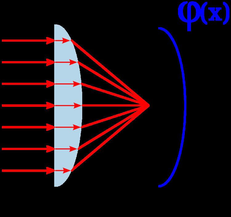
In order to understand how a spatial soliton can exist, we have to make some considerations about a simple convex lens. As shown in the picture on the right, an optical field approaches the lens and then it is focused. The effect of the lens is to introduce a non-uniform phase change that causes focusing. This phase change is a function of the space and can be represented with
The phase change can be expressed as the product of the phase constant and the width of the path the field has covered. We can write it as:
where
That's the way graded-index fibers work: the change in the refractive index introduces a focusing effect that can balance the natural diffraction of the field. If the two effects balance each other perfectly, then we have a confined field propagating within the fiber.
Spatial solitons are based on the same principle: the Kerr effect introduces a Self-phase modulation that changes the refractive index according to the intensity:
if
The optical waveguide the soliton creates while propagating is not only a mathematical model, but it actually exists and can be used to guide other waves at different frequencies. This way it is possible to let light interact with light at different frequencies (this is impossible in linear media).
Proof
An electric field is propagating in a medium showing optical Kerr effect, so the refractive index is given by:
we remember that the relationship between irradiance and electric field is (in the complex representation):
where
The field is propagating in the
where
where it was pointed out clearly that the refractive index (thus the phase constant) depends on intensity. If we replace the expression of the electric field in the equation, assuming that the envelope
the equation becomes:
Let us introduce an approximation that is valid because the nonlinear effects are always much smaller than the linear ones:
now we express the intensity in terms of the electric field:
the equation becomes:
We will now assume
The equation becomes:
this is a common equation known as nonlinear Schrödinger equation. From this form, we can understand the physical meaning of the parameter N:
For
where sech is the hyperbolic secant. It still depends on z, but only in phase, so the shape of the field will not change during propagation.
For
It does change its shape during propagation, but it is a periodic function of z with period
For soliton solutions, N must be an integer and it is said to be the order or the soliton. For higher values of N, there are no closed form expressions, but the solitons exist and they are all periodic with different periods. Their shape can easily be expressed only immediately after generation:
on the right there is the plot of the second order soliton: at the beginning it has a shape of a sech, then the maximum amplitude increases and then comes back to the sech shape. Since high intensity is necessary to generate solitons, if the field increases its intensity even further the medium could be damaged.
The condition to be solved if we want to generate a fundamental soliton is obtained expressing N in terms of all the known parameters and then putting
that, in terms of maximum irradiance value becomes:
in most of the cases, the two variables that can be changed are the maximum intensity
Curiously, higher-order solitons can attain complicated shapes before returning exactly to their initial shape at the end of the soliton period. In the picture of various solitons, the spectrum (left) and time domain (right) are shown at varying distances of propagation (vertical axis) in an idealized nonlinear medium. This shows how a laser pulse might behave as it travels in a medium with the properties necessary to support fundamental solitons. In practice, in order to reach the very high peak intensity needed to achieve nonlinear effects, laser pulses may be coupled into optical fibers such as photonic-crystal fiber with highly confined propagating modes. Those fibers have more complicated dispersion and other characteristics which depart from the analytical soliton parameters.
Generation of spatial solitons
The first experiment on spatial optical solitons was reported in 1974 by Ashkin and Bjorkholm in a cell filled with sodium vapor. The field was then revisited in experiments at Limoges University in liquid carbon disulphide and expanded in the early '90s with the first observation of solitons in photorefractive crystals, glass, semiconductors and polymers. During the last decades numerous findings have been reported in various materials, for solitons of different dimensionality, shape, spiralling, colliding, fusing, splitting, in homogeneous media, periodic systems, and waveguides. Spatials solitons are also referred to as self-trapped optical beams and their formation is normally also accompanied by a self-written waveguide. In nematic liquid crystals, spatial solitons are also referred to as nematicons.
Temporal solitons
The main problem that limits transmission bit rate in optical fibres is group velocity dispersion. It is because generated impulses have a non-zero bandwidth and the medium they are propagating through has a refractive index that depends on frequency (or wavelength). This effect is represented by the group delay dispersion parameter D; using it, it is possible to calculate exactly how much the pulse will widen:
where L is the length of the fibre and
Consider the picture on the right. On the left there is a standard Gaussian pulse, that's the envelope of the field oscillating at a defined frequency. We assume that the frequency remains perfectly constant during the pulse.
Now we let this pulse propagate through a fibre with
Now let us assume we have a medium that shows only nonlinear Kerr effect but its refractive index does not depend on frequency: such a medium does not exist, but it's worth considering it to understand the different effects.
The phase of the field is given by:
the frequency (according to its definition) is given by:
this situation is represented in the picture on the left. At the beginning of the pulse the frequency is lower, at the end it's higher. After the propagation through our ideal medium, we will get a chirped pulse with no broadening because we have neglected dispersion.
Coming back to the first picture, we see that the two effects introduce a change in frequency in two different opposite directions. It is possible to make a pulse so that the two effects will balance each other. Considering higher frequencies, linear dispersion will tend to let them propagate faster, while nonlinear Kerr effect will slow them down. The overall effect will be that the pulse does not change while propagating: such pulses are called temporal solitons.
History of temporal solitons
In 1973, Akira Hasegawa and Fred Tappert of AT&T Bell Labs were the first to suggest that solitons could exist in optical fibres, due to a balance between self-phase modulation and anomalous dispersion. Also in 1973 Robin Bullough made the first mathematical report of the existence of optical solitons. He also proposed the idea of a soliton-based transmission system to increase performance of optical telecommunications.
Solitons in a fibre optic system are described by the Manakov equations.
In 1987, P. Emplit, J.P. Hamaide, F. Reynaud, C. Froehly and A. Barthelemy, from the Universities of Brussels and Limoges, made the first experimental observation of the propagation of a dark soliton, in an optical fiber.
In 1988, Linn Mollenauer and his team transmitted soliton pulses over 4,000 kilometres using a phenomenon called the Raman effect, named for the Indian scientist Sir C. V. Raman who first described it in the 1920s, to provide optical gain in the fibre.
In 1991, a Bell Labs research team transmitted solitons error-free at 2.5 gigabits over more than 14,000 kilometres, using erbium optical fibre amplifiers (spliced-in segments of optical fibre containing the rare earth element erbium). Pump lasers, coupled to the optical amplifiers, activate the erbium, which energizes the light pulses.
In 1998, Thierry Georges and his team at France Télécom R&D Centre, combining optical solitons of different wavelengths (wavelength division multiplexing), demonstrated a data transmission of 1 terabit per second (1,000,000,000,000 units of information per second).
Proof
An electric field is propagating in a medium showing optical Kerr effect through a guiding structure (such as an optical fibre) that limits the power on the xy plane. If the field is propagating towards z with a phase constant
where
Since in the medium there is a dispersion we can not neglect, the relationship between the electric field and its polarization is given by a convolution integral. Anyway, using a representation in the Fourier domain, we can replace the convolution with a simple product, thus using standard relationships that are valid in simpler media. We Fourier-transform the electric field using the following definition:
Using this definition, a derivative in the time domain corresponds to a product in the Fourier domain:
the complete expression of the field in the frequency domain is:
Now we can solve Helmholtz equation in the frequency domain:
we decide to express the phase constant with the following notation:
where we assume that
where, as known:
we put the expression of the electric field in the equation and make some calculations. If we assume the slowly varying envelope approximation:
we get:
we are ignoring the behavior in the xy plane, because it is already known and given by
replacing this in the equation we get simply:
Now we want to come back in the time domain. Expressing the products by derivatives we get the duality:
we can write the non linear component in terms of the irradiance or amplitude of the field:
for duality with the spatial soliton, we define:
and this symbol has the same meaning of the previous case, even if the context is different. The equation becomes:
We know that the impulse is propagating along the z axis with a group velocity given by
and the equation becomes:
We now further assume that the medium where the field is propagating in shows anomalous dispersion, i.e.
replacing those in the equation we get:
that is exactly the same equation we have obtained in the previous case. The first order soliton is given by:
the same considerations we have made are valid in this case. The condition
or, in terms of irradiance:
or we can express it in terms of power if we introduce an effective area
Stability of solitons
We have described what optical solitons are and, using mathematics, we have seen that, if we want to create them, we have to create a field with a particular shape (just sech for the first order) with a particular power related to the duration of the impulse. But what if we are a bit wrong in creating such impulses? Adding small perturbations to the equations and solving them numerically, it is possible to show that mono-dimensional solitons are stable. They are often referred as (1 + 1) D solitons, meaning that they are limited in one dimension (x or t, as we have seen) and propagate in another one (z).
If we create such a soliton using slightly wrong power or shape, then it will adjust itself until it reaches the standard sech shape with the right power. Unfortunately this is achieved at the expense of some power loss, that can cause problems because it can generate another non-soliton field propagating together with the field we want. Mono-dimensional solitons are very stable: for example, if
The only way to create a (1 + 1) D spatial soliton is to limit the field on the y axis using a dielectric slab, then limiting the field on x using the soliton.
On the other hand, (2 + 1) D spatial solitons are unstable, so any small perturbation (due to noise, for example) can cause the soliton to diffract as a field in a linear medium or to collapse, thus damaging the material. It is possible to create stable (2 + 1) D spatial solitons using saturating nonlinear media, where the Kerr relationship
If we consider the propagation of shorter (temporal) light pulses or over a longer distance, we need to consider higher-order corrections and therefore the pulse carrier envelope is governed by the higher-order nonlinear Schrödinger equation (HONSE) for which there are some specialized (analytical) soliton solutions.
Effect of power losses
As we have seen, in order to create a soliton it is necessary to have the right power when it is generated. If there are no losses in the medium, then we know that the soliton will keep on propagating forever without changing shape (1st order) or changing its shape periodically (higher orders). Unfortunately any medium introduces losses, so the actual behaviour of power will be in the form:
this is a serious problem for temporal solitons propagating in fibers for several kilometers. Let us consider what happens for the temporal soliton, generalization to the spatial ones is immediate. We have proved that the relationship between power
if the power changes, the only thing that can change in the second part of the relationship is
the width of the impulse grows exponentially to balance the losses! this relationship is true as long as the soliton exists, i.e. until this perturbation is small, so it must be
Generation of soliton pulse
Experiments have been carried out to analyse the effect of high frequency (20 MHz-1 GHz) external magnetic field induced nonlinear Kerr effect on Single mode optical fibre of considerable length (50-100m) to compensate group velocity dispersion (GVD) and subsequent evolution of soliton pulse ( peak energy, narrow, secant hyperbolic pulse). Generation of soliton pulse in fibre is an obvious conclusion as self phase modulation due to high energy of pulse offset GVD, whereas the evolution length is 2000 km. (the laser wavelength chosen greater than 1.3 micrometers). Moreover, peak soliton pulse is of period 1-3ps so that it is safely accommodated in the optical bandwidth. Once soliton pulse is generated it is least dispersed over thousands of kilometres length of fibre limiting the number of repeater stations.
Dark solitons
In the analysis of both types of solitons we have assumed particular conditions about the medium:
Is it possible to obtain solitons if those conditions are not verified? if we assume
This equation has soliton-like solutions. For the first order (N=1):
The plot of
It is a soliton, in the sense that it propagates without changing its shape, but it is not made by a normal pulse; rather, it is a lack of energy in a continuous time beam. The intensity is constant, but for a short time during which it jumps to zero and back again, thus generating a "dark pulse"'. Those solitons can actually be generated introducing short dark pulses in much longer standard pulses. Dark solitons are more difficult to handle than standard solitons, but they have shown to be more stable and robust to losses.