Suvarna Garge (Editor)

Skewed generalized t distribution

Updated on
Edit
Like
Comment
Share on FacebookTweet on TwitterShare on LinkedInShare on Reddit
Skewed generalized t distribution


In probability and statistics, the skewed generalized “t” distribution is a family of continuous probability distributions. The distribution was first introduced by Panayiotis Theodossiou in 1998. The distribution has since been used in different applications. There are different parameterizations for the skewed generalized t distribution, which we account for in this article.

Contents

Probability density function

f S G T ( x ; μ , σ , λ , p , q ) = p 2 v σ q 1 / p B ( 1 p , q ) ( | x μ + m | p q ( v σ ) p ( λ s i g n ( x μ + m ) + 1 ) p + 1 ) 1 p + q

where B is the beta function, μ is the location parameter, σ > 0 is the scale parameter, 1 < λ < 1 is the skewness parameter, and p > 0 and q > 0 are the parameters that control the kurtosis. Note that m and v are not parameters, but functions of the other parameters that are used here to scale or shift the distribution appropriately to match the various parameterizations of this distribution.

In the original parameterization of the skewed generalized t distribution,

m = 2 v σ λ q 1 p B ( 2 p , q 1 p ) B ( 1 p , q )

and

v = q 1 p ( 3 λ 2 + 1 ) B ( 3 p , q 2 p ) B ( 1 p , q ) 4 λ 2 B ( 2 p , q 1 p ) 2 B ( 1 p , q ) 2 .

These values for m and v yield a distribution with mean of μ if p q > 1 and a variance of σ 2 if p q > 2 . In order for m to take on this value however, it must be the case that p q > 1 . Similarly, for v to equal the above value, p q > 2 .

The parameterization that yields the simplest functional form of the probability density function sets m = 0 and v = 1 . This gives a mean of

μ + 2 v σ λ q 1 p B ( 2 p , q 1 p ) B ( 1 p , q )

and a variance of

σ 2 q 2 p ( ( 3 λ 2 + 1 ) B ( 3 p , q 2 p ) B ( 1 p , q ) 4 λ 2 B ( 2 p , q 1 p ) 2 B ( 1 p , q ) 2 )

The λ parameter controls the skewness of the distribution. To see this, let M denote the mode of the distribution, and note that

M f S G T ( x ; μ , σ , λ , p , q ) d x = 1 λ 2

Since 1 < λ < 1 , the probability left of the mode, and therefore right of the mode as well, can equal any value in (0,1) depending on the value of λ . Thus the skewed generalized t distribution can be highly skewed as well as symmetric. If 1 < λ < 0 , then the distribution is negatively skewed. If 0 < λ < 1 , then the distribution is positively skewed. If λ = 0 , then the distribution is symmetric.

Finally, p and q control the kurtosis of the distribution. As p and q get smaller, the kurtosis increases (i.e. becomes more leptokurtic). Large values of p and q yield a distribution that is more platykurtic.

Moments

Let X be a random variable distributed with the skewed generalized t distribution.The h t h moment (i.e. E [ ( X E ( X ) ) h ] ), for p q > h , is: r = 0 h ( h r ) ( ( 1 + λ ) r + 1 + ( 1 ) r ( 1 λ ) r + 1 ) ( λ ) h r ( v σ ) h q h p B ( r + 1 p , q r p ) B ( 2 p , q 1 p ) h r 2 r h + 1 B ( 1 p , q ) h r + 1

The mean, for p q > 1 , is:

μ + 2 v σ λ q 1 p B ( 2 p , q 1 p ) B ( 1 p , q ) m

The variance (i.e. E [ ( X E ( X ) ) 2 ] ), for p q > 2 , is:

( v σ ) 2 q 2 p ( ( 3 λ 2 + 1 ) B ( 3 p , q 2 p ) B ( 1 p , q ) 4 λ 2 B ( 2 p , q 1 p ) 2 B ( 1 p , q ) 2 )

The skewness (i.e. E [ ( X E ( X ) ) 3 ] ), for p q > 3 , is:

2 q 3 / p λ ( v σ ) 3 B ( 1 p , q ) 3 ( 8 λ 2 B ( 2 p , q 1 p ) 3 3 ( 1 + 3 λ 2 ) B ( 1 p , q ) × B ( 2 p , q 1 p ) B ( 3 p , q 2 p ) + 2 ( 1 + λ 2 ) B ( 1 p , q ) 2 B ( 4 p , q 3 p ) )

The kurtosis (i.e. E [ ( X E ( X ) ) 4 ] ), for p q > 4 , is:

q 4 / p ( v σ ) 4 B ( 1 p , q ) 4 ( 48 λ 4 B ( 2 p , q 1 p ) 4 + 24 λ 2 ( 1 + 3 λ 2 ) B ( 1 p , q ) B ( 2 p , q 1 p ) 2 × B ( 3 p , q 2 p ) 32 λ 2 ( 1 + λ 2 ) B ( 1 p , q ) 2 B ( 2 p , q 1 p ) B ( 4 p , q 3 p ) + ( 1 + 10 λ 2 + 5 λ 4 ) B ( 1 p , q ) 3 B ( 5 p , q 4 p ) )

Special Cases

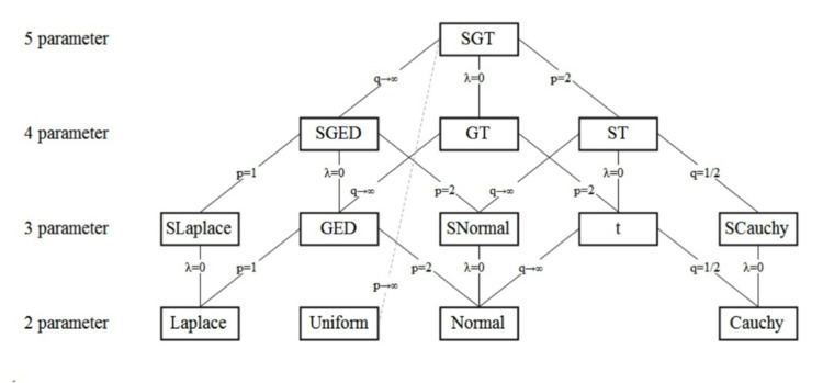
Special and limiting cases of the skewed generalized t distribution include the skewed generalized error distribution, the generalized t distribution introduced by McDonald and Newey, the skewed t proposed by Hansen, the skewed Laplace distribution, the generalized error distribution (also known as the generalized normal distribution), a skewed normal distribution, the student t distribution, the skewed Cauchy distribution, the Laplace distribution, the uniform distribution, the normal distribution, and the Cauchy distribution. The graphic below, adapted from Hansen, McDonald, and Newey, shows which parameters should be set to obtain some of the different special values of the skewed generalized t distribution.

skewed generalized error distribution

The Skewed Generalized Error Distribution has the pdf:

lim q f S G T ( x ; μ , σ , λ , p , q ) = f S G E D ( x ; μ , σ , λ , p ) = p e ( | x μ + m | v σ ( 1 + λ s i g n ( x μ + m ) ) ) p 2 v σ Γ ( 1 / p )

where

m = 2 2 p v σ λ Γ ( 1 2 + 1 p ) π

gives a mean of μ . Also

v = π Γ ( 1 p ) π ( 1 + 3 λ 2 ) Γ ( 3 p ) 16 1 p λ 2 Γ ( 1 2 + 1 p ) 2 Γ ( 1 p )

gives a variance of σ 2 .

generalized t distribution

The Generalized T Distribution has the pdf:

f S G T ( x ; μ , σ , λ = 0 , p , q ) = f G T ( x ; μ , σ , p , q ) = p 2 v σ q 1 / p B ( 1 p , q ) ( | x μ | p q ( v σ ) p + 1 ) 1 p + q

where

v = 1 q 1 / p B ( 1 p , q ) B ( 3 p , q 2 p ) )

gives a variance of σ 2 .

skewed t distribution

The Skewed T Distribution has the pdf:

f S G T ( x ; μ , σ , λ , p = 2 , q ) = f S T ( x ; μ , σ , λ , q ) = Γ ( 1 2 + q ) v σ ( π q ) 1 / 2 Γ ( q ) ( | x μ + m | 2 q ( v σ ) 2 ( λ s i g n ( x μ + m ) + 1 ) 2 + 1 ) 1 2 + q

where

m = 2 v σ λ q 1 / 2 Γ ( q 1 2 ) π 1 / 2 Γ ( q + 1 2 )

gives a mean of μ . Also

v = 1 q 1 / 2 ( 3 λ 2 + 1 ) ( 1 2 q 2 ) 4 λ 2 π ( Γ ( q 1 2 ) Γ ( q ) ) 2

gives a variance of σ 2 .

skewed Laplace distribution

The Skewed Laplace Distribution has the pdf:

lim q f S G T ( x ; μ , σ , λ , p = 1 , q ) = f S L a p l a c e ( x ; μ , σ , λ ) = e | x μ + m | v σ ( 1 + λ s i g n ( x μ + m ) ) 2 v σ

where

m = 2 v σ λ

gives a mean of μ . Also

v = [ 2 ( 1 + λ 2 ) ] 1 2

gives a variance of σ 2 .

generalized error distribution

The Generalized Error Distribution (also known as the generalized normal distribution) has the pdf:

lim q f S G T ( x ; μ , σ , λ = 0 , p , q ) = f G E D ( x ; μ , σ , p ) = p e ( | x μ | v σ ) p 2 v σ Γ ( 1 / p )

where

v = Γ ( 1 p ) Γ ( 3 p )

gives a variance of σ 2 .

skewed normal distribution

The Skewed Normal Distribution has the pdf:

lim q f S G T ( x ; μ , σ , λ , p = 2 , q ) = f S N o r m a l ( x ; μ , σ , λ ) = e ( | x μ + m | v σ ( 1 + λ s i g n ( x μ + m ) ) ) 2 v σ π

where

m = 2 v σ λ π

gives a mean of μ . Also

v = 2 π ( π 8 λ 2 + 3 π λ 2 )

gives a variance of σ 2 .

student's t-distribution

The Student's t-distribution has the pdf:

f S G T ( x ; μ = 0 , σ = 1 , λ = 0 , p = 2 , q = d / 2 ) = f T ( x ; d ) = Γ ( d + 1 2 ) ( π d ) 1 / 2 Γ ( d / 2 ) ( x 2 d + 1 ) d + 1 2

Note that we substituted v = 2 .

skewed Cauchy distribution

The Skewed Cauchy Distribution has the pdf:

f S G T ( x ; μ , σ , λ , p = 2 , q = 1 / 2 ) = f S C a u c h y ( x ; μ , σ , λ ) = 1 σ π ( | x μ | 2 σ 2 ( λ s i g n ( x μ ) + 1 ) 2 + 1 )

Note that we substituted v = 2 and m = 0 .

Laplace distribution

The Laplace distribution has the pdf:

lim q f S G T ( x ; μ , σ , λ = 0 , p = 1 , q ) = f L a p l a c e ( x ; μ , σ ) = e | x μ | σ 2 σ

Note that we substituted v = 1 .

Uniform Distribution

The Uniform distribution has the pdf:

lim p f S G T ( x ; μ , σ , λ , p , q ) = f ( x ) = { 1 2 v σ | x μ | < v σ 0 o t h e r w i s e

Thus the standard uniform parameterization is obtained if μ = a + b 2 , v = 1 , and σ = b a 2 .

Normal distribution

The Normal distribution has the pdf:

lim q f S G T ( x ; μ , σ , λ = 0 , p = 2 , q ) = f N o r m a l ( x ; μ , σ ) = e ( | x μ | v σ ) 2 v σ π

where

v = 2

gives a variance of σ 2 .

Cauchy Distribution

The Cauchy distribution has the pdf:

f S G T ( x ; μ , σ , λ = 0 , p = 2 , q = 1 / 2 ) = f C a u c h y ( x ; μ , σ ) = 1 σ π ( ( x μ σ ) 2 + 1 )

Note that we substituted v = 2 .

References

Skewed generalized t distribution Wikipedia