Skellam distribution - Alchetron, The Free Social Encyclopedia

Median N/A

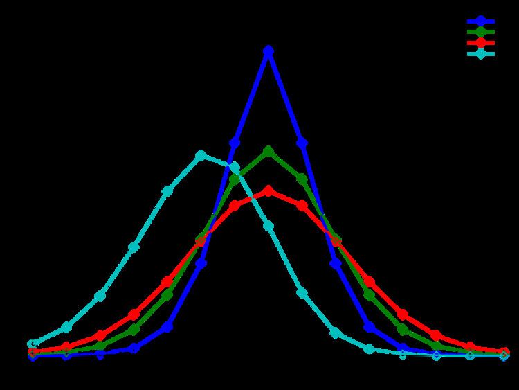Parameters μ 1 ≥ 0 , μ 2 ≥ 0 {\displaystyle \mu _{1}\geq 0,~~\mu _{2}\geq 0} Support { … , − 2 , − 1 , 0 , 1 , 2 , … } {\displaystyle \{\ldots ,-2,-1,0,1,2,\ldots \}} pmf e − ( μ 1 + μ 2 ) ( μ 1 μ 2 ) k / 2 I k ( 2 μ 1 μ 2 ) {\displaystyle e^{-(\mu _{1}\!+\!\mu _{2})}\left({\frac {\mu _{1}}{\mu _{2}}}\right)^{k/2}\!\!I_{k}(2{\sqrt {\mu _{1}\mu _{2}}})} Mean μ 1 − μ 2 {\displaystyle \mu _{1}-\mu _{2}\,} Variance μ 1 + μ 2 {\displaystyle \mu _{1}+\mu _{2}\,}

The Skellam distribution is the discrete probability distribution of the difference N 1 − N 2 of two statistically independent random variables N 1 and N 2 , each Poisson-distributed with respective expected values μ 1 and μ 2 It is useful in describing the statistics of the difference of two images with simple photon noise, as well as describing the point spread distribution in sports where all scored points are equal, such as baseball, hockey and soccer.

The distribution is also applicable to a special case of the difference of dependent Poisson random variables, but just the obvious case where the two variables have a common additive random contribution which is cancelled by the differencing: see Karlis & Ntzoufras (2003) for details and an application.

The probability mass function for the Skellam distribution for a difference K = N 1 − N 2 between two independent Poisson-distributed random variables with means μ 1 and μ 2 is given by:

p ( k ; μ 1 , μ 2 ) = Pr { K = k } = e − ( μ 1 + μ 2 ) ( μ 1 μ 2 ) k / 2 I k ( 2 μ 1 μ 2 )

where I_k(z) is the modified Bessel function of the first kind. Since k is an integer we have that I_k(z)=I_|k|(z).

Derivation

Note that the probability mass function of a Poisson-distributed random variable with mean μ is given by

p ( k ; μ ) = μ k k ! e − μ .

for k ≥ 0 (and zero otherwise). The Skellam probability mass function for the difference of two independent counts K = N 1 − N 2 is the convolution of two Poisson distributions: (Skellam, 1946)

p ( k ; μ 1 , μ 2 ) = ∑ n = − ∞ ∞ p ( k + n ; μ 1 ) p ( n ; μ 2 ) = e − ( μ 1 + μ 2 ) ∑ n = m a x ( 0 , − k ) ∞ μ 1 k + n μ 2 n n ! ( k + n ) !

Since the Poisson distribution is zero for negative values of the count ( p ( N < 0 ; μ ) = 0 ) , the second sum is only taken for those terms where n >= 0 and n + k >= 0 . It can be shown that the above sum implies that

p ( k ; μ 1 , μ 2 ) p ( − k ; μ 1 , μ 2 ) = ( μ 1 μ 2 ) k

so that:

p ( k ; μ 1 , μ 2 ) = e − ( μ 1 + μ 2 ) ( μ 1 μ 2 ) k / 2 I | k | ( 2 μ 1 μ 2 )

where I _k(z) is the modified Bessel function of the first kind. The special case for μ 1 = μ 2 ( = μ ) is given by Irwin (1937):

p ( k ; μ , μ ) = e − 2 μ I | k | ( 2 μ ) .

Note also that, using the limiting values of the modified Bessel function for small arguments, we can recover the Poisson distribution as a special case of the Skellam distribution for μ 2 = 0 .

Properties

As it is a discrete probability function, the Skellam probability mass function is normalized:

∑ k = − ∞ ∞ p ( k ; μ 1 , μ 2 ) = 1 .

We know that the probability generating function (pgf) for a Poisson distribution is:

G ( t ; μ ) = e μ ( t − 1 ) .

It follows that the pgf, G ( t ; μ 1 , μ 2 ) , for a Skellam probability mass function will be:

G ( t ; μ 1 , μ 2 ) = ∑ k = 0 ∞ p ( k ; μ 1 , μ 2 ) t k = G ( t ; μ 1 ) G ( 1 / t ; μ 2 ) = e − ( μ 1 + μ 2 ) + μ 1 t + μ 2 / t .

Notice that the form of the probability generating function implies that the distribution of the sums or the differences of any number of independent Skellam-distributed variables are again Skellam-distributed. It is sometimes claimed that any linear combination of two Skellam-distributed variables are again Skellam-distributed, but this is clearly not true since any multiplier other than ± 1 would change the support of the distribution and alter the pattern of moments in a way that no Skellam distribution can satisfy.

The moment-generating function is given by:

M ( t ; μ 1 , μ 2 ) = G ( e t ; μ 1 , μ 2 ) = ∑ k = 0 ∞ t k k ! m k

which yields the raw moments m_k . Define:

Δ = d e f μ 1 − μ 2 μ = d e f ( μ 1 + μ 2 ) / 2.

Then the raw moments m_k are

m 1 = Δ m 2 = 2 μ + Δ 2 m 3 = Δ ( 1 + 6 μ + Δ 2 )

The central moments M _k are

M 2 = 2 μ , M 3 = Δ , M 4 = 2 μ + 12 μ 2 .

The mean, variance, skewness, and kurtosis excess are respectively:

E ( n ) = Δ σ 2 = 2 μ γ 1 = Δ / ( 2 μ ) 3 / 2 γ 2 = 1 / 2 μ .

The cumulant-generating function is given by:

K ( t ; μ 1 , μ 2 ) = d e f ln ⁡ ( M ( t ; μ 1 , μ 2 ) ) = ∑ k = 0 ∞ t k k ! κ k

which yields the cumulants:

κ 2 k = 2 μ κ 2 k + 1 = Δ .

For the special case when μ₁ = μ₂, an asymptotic expansion of the modified Bessel function of the first kind yields for large μ:

p ( k ; μ , μ ) ∼ 1 4 π μ [ 1 + ∑ n = 1 ∞ ( − 1 ) n { 4 k 2 − 1 2 } { 4 k 2 − 3 2 } ⋯ { 4 k 2 − ( 2 n − 1 ) 2 } n ! 2 3 n ( 2 μ ) n ] .

(Abramowitz & Stegun 1972, p. 377). Also, for this special case, when k is also large, and of order of the square root of 2μ, the distribution tends to a normal distribution:

p ( k ; μ , μ ) ∼ e − k 2 / 4 μ 4 π μ .

These special results can easily be extended to the more general case of different means.

The following recurrence relation holds. Let P ( k ) = p ( k ; μ 1 , μ 2 ) be the probability mass function for a Skellam-distributed random variable with parameters μ 1 and μ 2 . Then

{ − μ 1 P ( k ) + μ 2 P ( k + 2 ) + ( k + 1 ) P ( k + 1 ) = 0 , P ( 0 ) = e − μ 1 − μ 2 0 F ~ 1 ( ; 1 ; μ 1 μ 2 ) , P ( 1 ) = e − μ 1 − μ 2 μ 1 0 F ~ 1 ( ; 2 ; μ 1 μ 2 ) }

where 0 F ~ 1 denotes the regularized hypergeometric function.

Bounds on weight above zero

If X ∼ S k e l l a m ( μ 1 , μ 2 ) , with μ 1 < μ 2 , then

Details can be found in Poisson distribution#Poisson Races

References

Skellam distribution Wikipedia

(Text) CC BY-SA

Contents

Derivation

Properties

Bounds on weight above zero

References