Simpson's paradox

UC Berkeley gender bias

One of the best-known examples of Simpson's paradox is a study of gender bias among graduate school admissions to University of California, Berkeley. The admission figures for the fall of 1973 showed that men applying were more likely than women to be admitted, and the difference was so large that it was unlikely to be due to chance.

But when examining the individual departments, it appeared that six out of 85 departments were significantly biased against men, whereas only four were significantly biased against women. In fact, the pooled and corrected data showed a "small but statistically significant bias in favor of women." The data from the six largest departments is listed below.

The research paper by Bickel et al. concluded that women tended to apply to competitive departments with low rates of admission even among qualified applicants (such as in the English Department), whereas men tended to apply to less-competitive departments with high rates of admission among the qualified applicants (such as in engineering and chemistry). The conditions under which the admissions' frequency data from specific departments constitute a proper defense against charges of discrimination are formulated in the book Causality by Pearl.

Kidney stone treatment

This is a real-life example from a medical study comparing the success rates of two treatments for kidney stones.

The table below shows the success rates and numbers of treatments for treatments involving both small and large kidney stones, where Treatment A includes all open surgical procedures and Treatment B is percutaneous nephrolithotomy (which involves only a small puncture). The numbers in parentheses indicate the number of success cases over the total size of the group. (For example, 93% equals 81 divided by 87.)

The paradoxical conclusion is that treatment A is more effective when used on small stones, and also when used on large stones, yet treatment B is more effective when considering both sizes at the same time. In this example the "lurking" variable (or confounding variable) is the severity of the case (represented by the doctors' treatment decision trend of favoring B for less severe cases), which was not previously known to be important until its effects were included.

Which treatment is considered better is determined by an inequality between two ratios (successes/total). The reversal of the inequality between the ratios, which creates Simpson's paradox, happens because two effects occur together:

1. The sizes of the groups, which are combined when the lurking variable is ignored, are very different. Doctors tend to give the severe cases (large stones) the better treatment (A), and the milder cases (small stones) the inferior treatment (B). Therefore, the totals are dominated by groups 3 and 2, and not by the two much smaller groups 1 and 4.
2. The lurking variable has a large effect on the ratios; i.e., the success rate is more strongly influenced by the severity of the case than by the choice of treatment. Therefore, the group of patients with large stones using treatment A (group 3) does worse than the group with small stones (groups 1 and 2), even if the latter used the inferior treatment B (group 2).

Based on these effects, the paradoxical result is seen to arise by suppression of the causal effect of the severity of the case on successful treatment. The paradoxical result can be rephrased more accurately as follows: When the less effective treatment (B) is applied more frequently to less severe cases, it can appear to be a more effective treatment.

Low birth weight paradox

The low birth weight paradox is an apparently paradoxical observation relating to the birth weights and mortality of children born to tobacco smoking mothers. As a usual practice, babies weighing less than a certain amount (which varies between different countries) have been classified as having low birth weight. In a given population, babies with low birth weights have had a significantly higher infant mortality rate than others. Normal birth weight infants of smokers have about the same mortality rate as normal birth weight infants of non-smokers, and low birth weight infants of smokers have a much lower mortality rate than low birth weight infants of non-smokers, but infants of smokers overall have a much higher mortality rate than infants of non-smokers. This is because many more infants of smokers are low birth weight, and low birth weight babies have a much higher mortality rate than normal birth weight babies. However, some other causes of low birth weight carry a much higher infant mortality rate.

Batting averages

A common example of Simpson's Paradox involves the batting averages of players in professional baseball. It is possible for one player to have a higher batting average than another player each year for a number of years, but to have a lower batting average across all of those years. This phenomenon can occur when there are large differences in the number of at-bats between the years. (The same situation applies to calculating batting averages for the first half of the baseball season, and during the second half, and then combining all of the data for the season's batting average.)

A real-life example is provided by Ken Ross and involves the batting average of two baseball players, Derek Jeter and David Justice, during the years 1995 and 1996:

In both 1995 and 1996, Justice had a higher batting average (in bold type) than Jeter did. However, when the two baseball seasons are combined, Jeter shows a higher batting average than Justice. According to Ross, this phenomenon would be observed about once per year among the possible pairs of interesting baseball players. In this particular case, the Simpson's Paradox can still be observed if the year 1997 is also taken into account:

The Jeter and Justice example of Simpson's paradox was referred to in the "Conspiracy Theory" episode of the television series Numb3rs, though a chart shown omitted some of the data, and listed the 1996 averages as 1995.

Correlation between variables

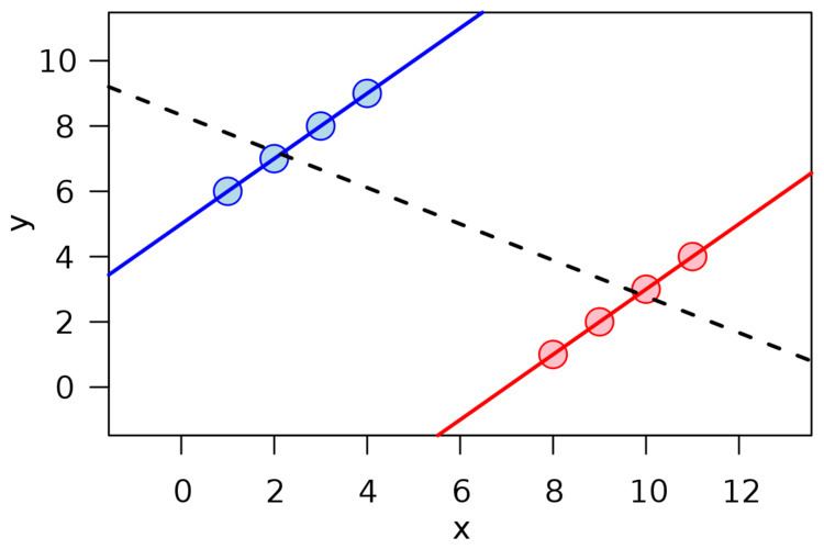
Simpson's paradox can also arise in correlations, in which two variables appear to have (say) a positive correlation towards one another, when in fact they have a negative correlation, the reversal having been brought about by a "lurking" confounder. Berman et al. give an example from economics, where a dataset suggests overall demand is positively correlated with price (that is, higher prices lead to more demand), in contradiction of expectation. Analysis reveals time to be the confounding variable: plotting both price and demand against time reveals the expected negative correlation over various periods, which then reverses to become positive if the influence of time is ignored by simply plotting demand against price.

Description

Suppose two people, Lisa and Bart, each edit articles for two weeks. In the first week, Lisa fails to improve the only article she edited, and Bart improves 1 of the 4 articles he edited. In the second week, Lisa improves 3 of 4 articles she edited, while Bart improves the only article he edited.

Both times Bart improved a higher percentage of articles than Lisa, but the actual number of articles each edited (the bottom number of their ratios, also known as the sample size) were not the same for both of them either week. When the totals for the two weeks are added together, Bart and Lisa's work can be judged from an equal sample size; i.e., the total number of articles edited by each. Looked at in this more accurate manner, Lisa's ratio is higher and, therefore, so is her percentage. Also when the two tests are combined using a weighted average, overall, Lisa has improved a much higher percentage than Bart because the quality modifier had a significantly higher percentage. Therefore, like other paradoxes, it only appears to be a paradox because of incorrect assumptions, incomplete or misguided information, or a lack of understanding a particular concept.

This imagined paradox is caused when the percentage is provided but not the ratio. In this example, if only the 25% in the first week for Bart was provided but not the ratio (1:4), it would distort the information and so cause the imagined paradox. Even though Bart's percentage is higher for the first and second week, when two weeks of articles is combined, overall Lisa had improved a greater proportion, 60% of the 5 total articles. Lisa's proportional total of articles improved exceeds Bart's total.

Vector interpretation

Simpson's paradox can also be illustrated using the 2-dimensional vector space. A success rate of p q (i.e., successes/attempts) can be represented by a vector A → = ( q , p ) , with a slope of p q . A larger slope, meaning a steeper vector direction, represents then a more successful week. If two rates p 1 q 1 and p 2 q 2 are combined, as in the examples given above, the result can be represented by the sum of the vectors ( q 1 , p 1 ) and ( q 2 , p 2 ) , which according to the parallelogram rule is the vector ( q 1 + q 2 , p 1 + p 2 ) , with slope p 1 + p 2 q 1 + q 2 .

Simpson's paradox says that even if a vector L 1 → (in light brown in the figure) has a smaller slope than another vector B 1 → (in blue), and L 2 → has a smaller slope than B 2 → , the sum of the two vectors L 1 → + L 2 → can still have a larger slope than the sum of the two vectors B 1 → + B 2 → , as shown in the example.

Implications for decision making

The practical significance of Simpson's paradox surfaces in decision making situations where it poses the following dilemma: Which data should we consult in choosing an action, the aggregated or the partitioned? In the Kidney Stone example above, it is clear that if one is diagnosed with "Small Stones" or "Large Stones" the data for the respective subpopulation should be consulted and Treatment A would be preferred to Treatment B. But what if a patient is not diagnosed, and the size of the stone is not known; would it be appropriate to consult the aggregated data and administer Treatment B? This would stand contrary to common sense; a treatment that is preferred both under one condition and under its negation should also be preferred when the condition is unknown.

On the other hand, if the partitioned data is to be preferred a priori, what prevents one from partitioning the data into arbitrary sub-categories (say based on eye color or post-treatment pain) artificially constructed to yield wrong choices of treatments? Pearl shows that, indeed, in many cases it is the aggregated, not the partitioned data that gives the correct choice of action. Worse yet, given the same table, one should sometimes follow the partitioned and sometimes the aggregated data, depending on the story behind the data, with each story dictating its own choice. Pearl considers this to be the real paradox behind Simpson's reversal.

As to why and how a story, not data, should dictate choices, the answer is that it is the story which encodes the causal relationships among the variables. Once we explicate these relationships and represent them formally, we can test which partition gives the correct treatment preference. For example, if we represent causal relationships in a graph called "causal diagram" (see Bayesian networks), we can test whether nodes that represent the proposed partition intercept spurious paths in the diagram. This test, called "back-door," reduces Simpson's paradox to an exercise in graph theory (see page 7 of )

Psychology

Psychological interest in Simpson's paradox seeks to explain why people deem sign reversal to be impossible at first, offended by the idea that an action preferred both under one condition and under its negation should be rejected when the condition is unknown. The question is where people get this strong intuition from, and how it is encoded in the mind. Simpson's paradox demonstrates that this intuition cannot be derived from either classical logic or probability calculus alone, and thus led philosophers to speculate that it is supported by an innate causal logic that guides people in reasoning about actions and their consequences. Savage's sure-thing principle is an example of what such logic may entail. A qualified version of Savage's sure thing principle can indeed be derived from Pearl's do-calculus and reads: "An action A that increases the probability of an event B in each subpopulation C_i of C must also increase the probability of B in the population as a whole, provided that the action does not change the distribution of the subpopulations." This suggests that knowledge about actions and consequences is stored in a form resembling Causal Bayesian Networks.

Probability

A paper by Pavlides and Perlman presents a proof, due to Hadjicostas, that in a random 2 × 2 × 2 table with uniform distribution, Simpson's paradox will occur with a probability of exactly ¹/₆₀ A study by Kock suggests that the probability that Simpson’s paradox would occur at random in path models (i.e., models generated by path analysis (statistics)) with two predictors and one criterion variable is approximately 12.8 percent; slightly higher than 1 occurrence per 8 path models.

Related concepts