Semi supervised learning - Alchetron, the free social encyclopedia

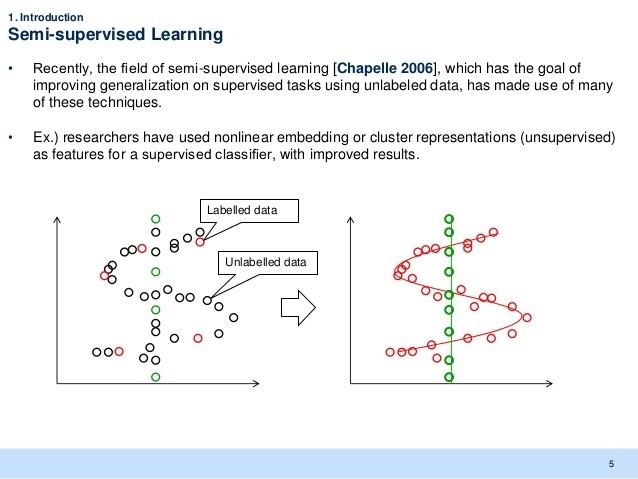
Semi-supervised learning is a class of supervised learning tasks and techniques that also make use of unlabeled data for training – typically a small amount of labeled data with a large amount of unlabeled data. Semi-supervised learning falls between unsupervised learning (without any labeled training data) and supervised learning (with completely labeled training data). Many machine-learning researchers have found that unlabeled data, when used in conjunction with a small amount of labeled data, can produce considerable improvement in learning accuracy. The acquisition of labeled data for a learning problem often requires a skilled human agent (e.g. to transcribe an audio segment) or a physical experiment (e.g. determining the 3D structure of a protein or determining whether there is oil at a particular location). The cost associated with the labeling process thus may render a fully labeled training set infeasible, whereas acquisition of unlabeled data is relatively inexpensive. In such situations, semi-supervised learning can be of great practical value. Semi-supervised learning is also of theoretical interest in machine learning and as a model for human learning.

As in the supervised learning framework, we are given a set of l independently identically distributed examples x 1 , … , x l ∈ X with corresponding labels y 1 , … , y l ∈ Y . Additionally, we are given u unlabeled examples x l + 1 , … , x l + u ∈ X . Semi-supervised learning attempts to make use of this combined information to surpass the classification performance that could be obtained either by discarding the unlabeled data and doing supervised learning or by discarding the labels and doing unsupervised learning.

Semi-supervised learning may refer to either transductive learning or inductive learning. The goal of transductive learning is to infer the correct labels for the given unlabeled data x l + 1 , … , x l + u only. The goal of inductive learning is to infer the correct mapping from X to Y .

Intuitively, we can think of the learning problem as an exam and labeled data as the few example problems that the teacher solved in class. The teacher also provides a set of unsolved problems. In the transductive setting, these unsolved problems are a take-home exam and you want to do well on them in particular. In the inductive setting, these are practice problems of the sort you will encounter on the in-class exam.

It is unnecessary (and, according to Vapnik's principle, imprudent) to perform transductive learning by way of inferring a classification rule over the entire input space; however, in practice, algorithms formally designed for transduction or induction are often used interchangeably.

Weka tutorial 26 semi supervised learning learning techniques

Assumptions used

In order to make any use of unlabeled data, we must assume some structure to the underlying distribution of data. Semi-supervised learning algorithms make use of at least one of the following assumptions.

Smoothness assumption

Points which are close to each other are more likely to share a label. (More accurately, this is a continuity assumption rather than a smoothness assumption.) This is also generally assumed in supervised learning and yields a preference for geometrically simple decision boundaries. In the case of semi-supervised learning, the smoothness assumption additionally yields a preference for decision boundaries in low-density regions, so that there are fewer points close to each other but in different classes.

Cluster assumption

The data tend to form discrete clusters, and points in the same cluster are more likely to share a label (although data sharing a label may be spread across multiple clusters). This is a special case of the smoothness assumption and gives rise to feature learning with clustering algorithms.

Manifold assumption

The data lie approximately on a manifold of much lower dimension than the input space. In this case we can attempt to learn the manifold using both the labeled and unlabeled data to avoid the curse of dimensionality. Then learning can proceed using distances and densities defined on the manifold.

The manifold assumption is practical when high-dimensional data are being generated by some process that may be hard to model directly, but which only has a few degrees of freedom. For instance, human voice is controlled by a few vocal folds, and images of various facial expressions are controlled by a few muscles. We would like in these cases to use distances and smoothness in the natural space of the generating problem, rather than in the space of all possible acoustic waves or images respectively.

History

The heuristic approach of self-training (also known as self-learning or self-labeling) is historically the oldest approach to semi-supervised learning, with examples of applications starting in the 1960s (see for instance Scudder (1965)).

The transductive learning framework was formally introduced by Vladimir Vapnik in the 1970s. Interest in inductive learning using generative models also began in the 1970s. A probably approximately correct learning bound for semi-supervised learning of a Gaussian mixture was demonstrated by Ratsaby and Venkatesh in 1995.

Semi-supervised learning has recently become more popular and practically relevant due to the variety of problems for which vast quantities of unlabeled data are available—e.g. text on websites, protein sequences, or images. For a review of recent work see a survey article by Zhu (2008).

Generative models

Generative approaches to statistical learning first seek to estimate p ( x | y ) , the distribution of data points belonging to each class. The probability p ( y | x ) that a given point x has label y is then proportional to p ( x | y ) p ( y ) by Bayes' rule. Semi-supervised learning with generative models can be viewed either as an extension of supervised learning (classification plus information about p ( x ) ) or as an extension of unsupervised learning (clustering plus some labels).

Generative models assume that the distributions take some particular form p ( x | y , θ ) parameterized by the vector θ . If these assumptions are incorrect, the unlabeled data may actually decrease the accuracy of the solution relative to what would have been obtained from labeled data alone. However, if the assumptions are correct, then the unlabeled data necessarily improves performance.

The unlabeled data are distributed according to a mixture of individual-class distributions. In order to learn the mixture distribution from the unlabeled data, it must be identifiable, that is, different parameters must yield different summed distributions. Gaussian mixture distributions are identifiable and commonly used for generative models.

The parameterized joint distribution can be written as p ( x , y | θ ) = p ( y | θ ) p ( x | y , θ ) by using the Chain rule. Each parameter vector θ is associated with a decision function f θ ( x ) = argmax y p ( y | x , θ ) . The parameter is then chosen based on fit to both the labeled and unlabeled data, weighted by λ :

argmax Θ ( log ⁡ p ( { x i , y i } i = 1 l | θ ) + λ log ⁡ p ( { x i } i = l + 1 l + u | θ ) )

Low-density separation

Another major class of methods attempts to place boundaries in regions where there are few data points (labeled or unlabeled). One of the most commonly used algorithms is the transductive support vector machine, or TSVM (which, despite its name, may be used for inductive learning as well). Whereas support vector machines for supervised learning seek a decision boundary with maximal margin over the labeled data, the goal of TSVM is a labeling of the unlabeled data such that the decision boundary has maximal margin over all of the data. In addition to the standard hinge loss ( 1 − y f ( x ) ) + for labeled data, a loss function ( 1 − | f ( x ) | ) + is introduced over the unlabeled data by letting y = sign ⁡ f ( x ) . TSVM then selects f ∗ ( x ) = h ∗ ( x ) + b from a reproducing kernel Hilbert space H by minimizing the regularized empirical risk:

f ∗ = argmin f ( ∑ i = 1 l ( 1 − y i f ( x i ) ) + + λ 1 ∥ h ∥ H 2 + λ 2 ∑ i = l + 1 l + u ( 1 − | f ( x i ) | ) + )

An exact solution is intractable due to the non-convex term ( 1 − | f ( x ) | ) + , so research has focused on finding useful approximations.

Other approaches that implement low-density separation include Gaussian process models, information regularization, and entropy minimization (of which TSVM is a special case).

Graph-based methods

Graph-based methods for semi-supervised learning use a graph representation of the data, with a node for each labeled and unlabeled example. The graph may be constructed using domain knowledge or similarity of examples; two common methods are to connect each data point to its k nearest neighbors or to examples within some distance ϵ . The weight W i j of an edge between x i and x j is then set to e − ∥ x i − x j ∥ 2 ϵ .

Within the framework of manifold regularization, the graph serves as a proxy for the manifold. A term is added to the standard Tikhonov regularization problem to enforce smoothness of the solution relative to the manifold (in the intrinsic space of the problem) as well as relative to the ambient input space. The minimization problem becomes

argmin f ∈ H ( 1 l ∑ i = 1 l V ( f ( x i ) , y i ) + λ A ∥ f ∥ H 2 + λ I ∫ M ∥ ∇ M f ( x ) ∥ 2 d p ( x ) )

where H is a reproducing kernel Hilbert space and M is the manifold on which the data lie. The regularization parameters λ A and λ I control smoothness in the ambient and intrinsic spaces respectively. The graph is used to approximate the intrinsic regularization term. Defining the graph Laplacian L = D − W where D i i = ∑ j = 1 l + u W i j and f the vector [ f ( x 1 ) … f ( x l + u ) ] , we have

f T L f = ∑ i , j = 1 l + u W i j ( f i − f j ) 2 ≈ ∫ M ∥ ∇ M f ( x ) ∥ 2 d p ( x ) .

The Laplacian can also be used to extend the supervised learning algorithms： regularized least squares and support vector machines (SVM) to semi-supervised versions Laplacian regularized least squares and Laplacian SVM.

Heuristic approaches

Some methods for semi-supervised learning are not intrinsically geared to learning from both unlabeled and labeled data, but instead make use of unlabeled data within a supervised learning framework. For instance, the labeled and unlabeled examples x 1 , … , x l + u may inform a choice of representation, distance metric, or kernel for the data in an unsupervised first step. Then supervised learning proceeds from only the labeled examples.

Self-training is a wrapper method for semi-supervised learning. First a supervised learning algorithm is trained based on the labeled data only. This classifier is then applied to the unlabeled data to generate more labeled examples as input for the supervised learning algorithm. Generally only the labels the classifier is most confident of are added at each step.

Co-training is an extension of self-training in which multiple classifiers are trained on different (ideally disjoint) sets of features and generate labeled examples for one another.

In human cognition

Human responses to formal semi-supervised learning problems have yielded varying conclusions about the degree of influence of the unlabeled data (for a summary see ). More natural learning problems may also be viewed as instances of semi-supervised learning. Much of human concept learning involves a small amount of direct instruction (e.g. parental labeling of objects during childhood) combined with large amounts of unlabeled experience (e.g. observation of objects without naming or counting them, or at least without feedback).

Human infants are sensitive to the structure of unlabeled natural categories such as images of dogs and cats or male and female faces. More recent work has shown that infants and children take into account not only the unlabeled examples available, but the sampling process from which labeled examples arise.

References

Semi-supervised learning Wikipedia

(Text) CC BY-SA

Contents