Secondary plot (kinetics) - Alchetron, the free social encyclopedia

In enzyme kinetics, a secondary plot uses the intercept or slope from several Lineweaver-Burk plots to find additional kinetic constants.

For example, when a set of v by [S] curves from an enzyme with a ping–pong mechanism (varying substrate A, fixed substrate B) are plotted in a Lineweaver–Burk plot, a set of parallel lines will be produced.

The following Michaelis–Menten equation relates the initial reaction rate v₀ to the substrate concentrations [A] and [B]:

1 v 0 = K M A v max [ A ] + K M B v max [ B ] + 1 v max

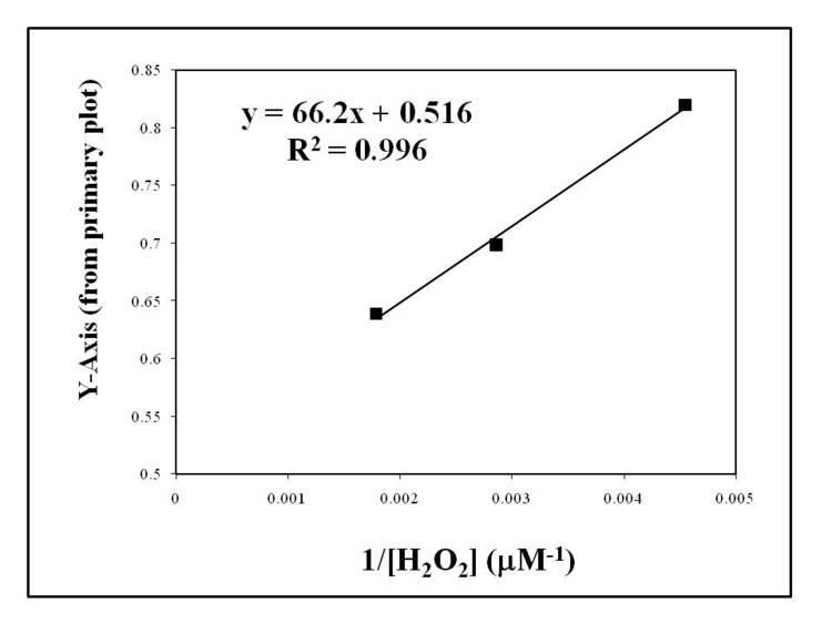
The y-intercept of this equation is equal to the following:

y-intercept = K M B v max [ B ] + 1 v max

The y-intercept is determined at several different fixed concentrations of substrate B (and varying substrate A). The y-intercept values are then plotted versus 1/[B] to determine the Michaelis constant for substrate B, K M B , as shown in the Figure to the right. The slope is equal to K M B divided by v max and the intercept is equal to 1 over v max .

Secondary Plot in Inhibition Studies

A secondary plot may also be used to find a specific inhbition constant, k_I.

For a competitive enzyme inhibitor, the apparent Michaelis constant is equal to the following:

apparent K m = K m × ( 1 + [ I ] K I )

The slope of the Lineweaver-Burk plot is therefore equal to:

slope = K m v max × ( 1 + [ I ] K I )

If one creates a secondary plot consisting of the slope values from several Lineweaver-Burk plots of varying inhibitor concentration [I], the competitive inhbition constant may be found. The slope of the secondary plot divided by the intercept is equal to 1/k_I. This method allows one to find the k_I constant, even when the Michaelis constant and v_max values are not known.

References

Secondary plot (kinetics) Wikipedia

(Text) CC BY-SA