Neha Patil (Editor)

Rosenbrock function

Updated on
Edit
Like
Comment
Share on FacebookTweet on TwitterShare on LinkedInShare on Reddit
Rosenbrock function

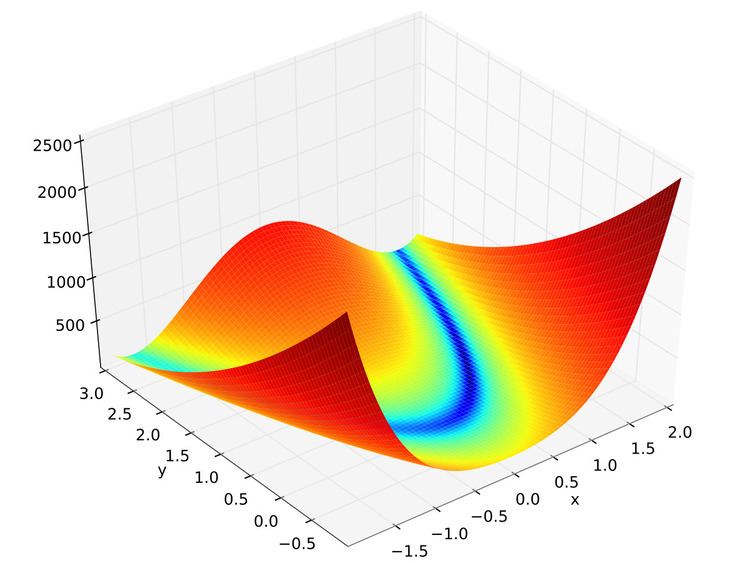
In mathematical optimization, the Rosenbrock function is a non-convex function used as a performance test problem for optimization algorithms introduced by Howard H. Rosenbrock in 1960. It is also known as Rosenbrock's valley or Rosenbrock's banana function.

Contents

The global minimum is inside a long, narrow, parabolic shaped flat valley. To find the valley is trivial. To converge to the global minimum, however, is difficult.

The function is defined by

f ( x , y ) = ( a x ) 2 + b ( y x 2 ) 2

It has a global minimum at ( x , y ) = ( a , a 2 ) , where f ( x , y ) = 0 . Usually a = 1 and b = 100 . Only in the trivial case of a = 0 is the function symmetric and the minimum at origo.

Multidimensional generalisations

Two variants are commonly encountered. One is the sum of N / 2 uncoupled 2D Rosenbrock problems,

f ( x ) = f ( x 1 , x 2 , , x N ) = i = 1 N / 2 [ 100 ( x 2 i 1 2 x 2 i ) 2 + ( x 2 i 1 1 ) 2 ] .

This variant is only defined for even N and has predictably simple solutions.

A more involved variant is

f ( x ) = i = 1 N 1 100 ( x i + 1 x i 2 ) 2 + ( 1 x i ) 2 where x = [ x 1 , , x N ] R N .

This variant has been shown to have exactly one minimum for N = 3 (at ( 1 , 1 , 1 ) ) and exactly two minima for 4 N 7 —the global minimum of all ones and a local minimum near ( x 1 , x 2 , , x N ) = ( 1 , 1 , , 1 ) . This result is obtained by setting the gradient of the function equal to zero, noticing that the resulting equation is a rational function of x . For small N the polynomials can be determined exactly and Sturm's theorem can be used to determine the number of real roots, while the roots can be bounded in the region of | x i | < 2.4 . For larger N this method breaks down due to the size of the coefficients involved.

Stationary points

Many of the stationary points of the function exhibit a regular pattern when plotted. This structure can be exploited to locate them.

An example of optimization

The Rosenbrock function can be efficiently optimized by adapting appropriate coordinate system without using any gradient information and without building local approximation models (in contrast to many derivate-free optimizers). The following figure illustrates an example of 2-dimensional Rosenbrock function optimization by adaptive coordinate descent from starting point x 0 = ( 3 , 4 ) . The solution with the function value 10 10 can be found after 325 function evaluations.

Using the Nelder–Mead method from starting point x 0 = ( 1 , 1 ) with a regular initial simplex a minimum is found with function value 1.36 10 10 after 185 function evaluations. The figure below visualizes the evolution of the algorithm.

References

Rosenbrock function Wikipedia


Similar Topics