Robust optimization

History

The origins of robust optimization date back to the establishment of modern decision theory in the 1950s and the use of worst case analysis and Wald's maximin model as a tool for the treatment of severe uncertainty. It became a discipline of its own in the 1970s with parallel developments in several scientific and technological fields. Over the years, it has been applied in statistics, but also in operations research, control theory, finance, portfolio management logistics, manufacturing engineering, chemical engineering, medicine, and computer science. In engineering problems, these formulations often take the name of "Robust Design Optimization", RDO or "Reliability Based Design Optimization", RBDO.

Example 1

Consider the following linear programming problem

where P is a given subset of R 2 .

What makes this a 'robust optimization' problem is the ∀ ( c , d ) ∈ P clause in the constraints. Its implication is that for a pair ( x , y ) to be admissible, the constraint c x + d y ≤ 10 must be satisfied by the worst ( c , d ) ∈ P pertaining to ( x , y ) , namely the pair ( c , d ) ∈ P that maximizes the value of c x + d y for the given value of ( x , y ) .

If the parameter space P is finite (consisting of finitely many elements), then this robust optimization problem itself is a linear programming problem: for each ( c , d ) ∈ P there is a linear constraint c x + d y ≤ 10 .

If P is not a finite set, then this problem is a linear semi-infinite programming problem, namely a linear programming problem with finitely many (2) decision variables and infinitely many constraints.

Classification

There are a number of classification criteria for robust optimization problems/models. In particular, one can distinguish between problems dealing with local and global models of robustness; and between probabilistic and non-probabilistic models of robustness. Modern robust optimization deals primarily with non-probabilistic models of robustness that are worst case oriented and as such usually deploy Wald's maximin models.

Local robustness

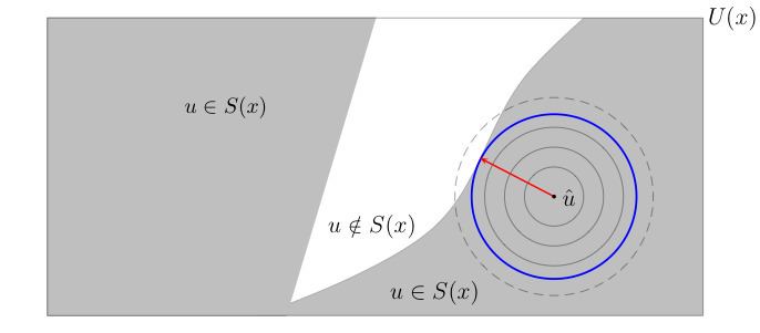
There are cases where robustness is sought against small perturbations in a nominal value of a parameter. A very popular model of local robustness is the radius of stability model:

where u ^ denotes the nominal value of the parameter, B ( ρ , u ^ ) denotes a ball of radius ρ centered at u ^ and S ( x ) denotes the set of values of u that satisfy given stability/performance conditions associated with decision x .

In words, the robustness (radius of stability) of decision x is the radius of the largest ball centered at u ^ all of whose elements satisfy the stability requirements imposed on x . The picture is this:

where the rectangle U ( x ) represents the set of all the values u associated with decision x .

Global robustness

Consider the simple abstract robust optimization problem

where U denotes the set of all possible values of u under consideration.

This is a global robust optimization problem in the sense that the robustness constraint g ( x , u ) ≤ b , ∀ u ∈ U represents all the possible values of u .

The difficulty is that such a "global" constraint can be too demanding in that there is no x ∈ X that satisfies this constraint. But even if such an x ∈ X exists, the constraint can be too "conservative" in that it yields a solution x ∈ X that generates a very small payoff f ( x ) that is not representative of the performance of other decisions in X . For instance, there could be an x ′ ∈ X that only slightly violates the robustness constraint but yields a very large payoff f ( x ′ ) . In such cases it might be necessary to relax a bit the robustness constraint and/or modify the statement of the problem.

Example 2

Consider the case where the objective is to satisfy a constraint g ( x , u ) ≤ b , . where x ∈ X denotes the decision variable and u is a parameter whose set of possible values in U . If there is no x ∈ X such that g ( x , u ) ≤ b , ∀ u ∈ U , then the following intuitive measure of robustness suggests itself:

where s i z e ( Y ) denotes an appropriate measure of the "size" of set Y . For example, if U is a finite set, then s i z e ( Y ) could be defined as the cardinality of set Y .

In words, the robustness of decision is the size of the largest subset of U for which the constraint g ( x , u ) ≤ b is satisfied for each u in this set. An optimal decision is then a decision whose robustness is the largest.

This yields the following robust optimization problem:

This intuitive notion of global robustness is not used often in practice because the robust optimization problems that it induces are usually (not always) very difficult to solve.

Example 3

Consider the robust optimization problem

where g is a real-valued function on X × U , and assume that there is no feasible solution to this problem because the robustness constraint g ( x , u ) ≤ b , ∀ u ∈ U is too demanding.

To overcome this difficulty, let N be a relatively small subset of U representing "normal" values of u and consider the following robust optimization problem:

Since N is much smaller than U , its optimal solution may not perform well on a large portion of U and therefore may not be robust against the variability of u over U .

One way to fix this difficulty is to relax the constraint g ( x , u ) ≤ b for values of u outside the set N in a controlled manner so that larger violations are allowed as the distance of u from N increases. For instance, consider the relaxed robustness constraint

where β ≥ 0 is a control parameter and d i s t ( u , N ) denotes the distance of u from N . Thus, for β = 0 the relaxed robustness constraint reduces back to the original robustness constraint. This yields the following (relaxed) robust optimization problem:

The function d i s t is defined in such a manner that

and

and therefore the optimal solution to the relaxed problem satisfies the original constraint g ( x , u ) ≤ b for all values of u in N . In addition, it also satisfies the relaxed constraint

outside N .

Non-probabilistic robust optimization models

The dominating paradigm in this area of robust optimization is Wald's maximin model, namely

where the max represents the decision maker, the min represents Nature, namely uncertainty, X represents the decision space and U ( x ) denotes the set of possible values of u associated with decision x . This is the classic format of the generic model, and is often referred to as minimax or maximin optimization problem. The non-probabilistic (deterministic) model has been and is being extensively used for robust optimization especially in the field of signal processing.

The equivalent mathematical programming (MP) of the classic format above is

Constraints can be incorporated explicitly in these models. The generic constrained classic format is

The equivalent constrained MP format is defined as:

Probabilistic robust optimization models

These models quantify the uncertainty in the "true" value of the parameter of interest by probability distribution functions. They have been traditionally classified as stochastic programming and stochastic optimization models.

Robust counterpart

The solution method to many robust program involves creating a deterministic equivalent, called the robust counterpart. The practical difficulty of a robust program depends on if its robust counterpart is computationally tractable.