Residence time distribution

Theory

The theory of residence time distributions generally begins with three assumptions:

1. the reactor is at steady-state,
2. transports at the inlet and the outlet takes place only by advection, and
3. the flow is incompressible.

The incompressibility assumption is not required, but compressible flows are more difficult to work with and less common in chemical processes. A further level of complexity is required for multi-phase reactors, where a separate RTD will describe the flow of each phase, for example bubbling air through a liquid.

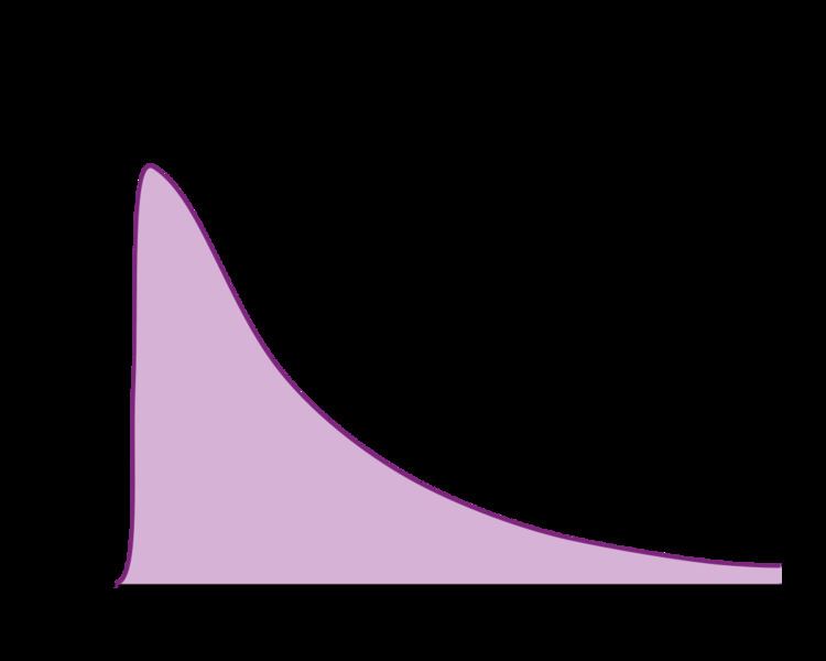
The distribution of residence times is represented by an exit age distribution, E ( t ) . The function E ( t ) has the units of time⁻¹ and is defined such that

The fraction of the fluid that spends a given duration, t inside the reactor is given by the value of E ( t ) d t .

The fraction of the fluid that leaves the reactor with an age less than t 1 is

The fraction of the fluid that leaves the reactor with an age greater than t 1 is

The average residence time is given by the first moment of the age distribution:

If there are no dead, or stagnant, zones within the reactor then t ¯ will be equal to τ , the residence time calculated from the total reactor volume and the volumetric flow rate of the fluid:

The higher order central moments can provide significant information about the behavior of the function E ( t ) . For example, the second central moment indicates the variance ( σ 2 ), the degree of dispersion around the mean.

The third central moment indicates the skewness of the RTD and the fourth central moment indicates the kurtosis (the "peakedness").

One can also define an internal age distribution I ( t ) that describes the reactor contents. This function has a similar definition as E ( t ) : the fraction of fluid within the reactor with an age of t is I ( t ) d t . As shown by Danckwerts, the relation between E ( t ) and I ( t ) can be found from the mass balance:

Determining the RTD Experimentally

Residence time distributions are measured by introducing a non-reactive tracer into the system at the inlet. The concentration of the tracer is changed according to a known function and the response is found by measuring the concentration of the tracer at the outlet. The selected tracer should not modify the physical characteristics of the fluid (equal density, equal viscosity) and the introduction of the tracer should not modify the hydrodynamic conditions. The Tracer chemical should have the properties, which are very essential for the RTD measurement are given below as follows- 1.) Non-reactive 2.) Easily detectable 3.) Properties similar to the reaction mixture 4.) Completely soluble 5.) Should not adsorb. In general, the change in tracer concentration will either be a pulse or a step. Other functions are possible, but they require more calculations to deconvolute the RTD curve, E ( t ) .

Pulse Experiments

This method required the introduction of a very small volume of concentrated tracer at the inlet of the reactor, such that it approaches the dirac delta function. Although an infinitely short injection cannot be produced, it can be made much smaller than the mean residence time of the vessel. If a mass of tracer, M , is introduced into a vessel of volume V and an expected residence time of τ , the resulting curve of C ( t ) can be transformed into a dimensionless residence time distribution curve by the following relation:

Step Experiments

The concentration of tracer in a step experiment at the reactor inlet changes abruptly from 0 to C 0 . The concentration of tracer at the outlet is measured and normalized to the concentration C 0 to obtain the non-dimensional curve F ( t ) which goes from 0 to 1:

The step- and pulse-responses of a reactor are related by the following:

The value of the mean residence time and the variance can also be deduced from the function F ( t ) :

A step experiment is often easier to perform than a pulse experiment, but it tends to smooth over some of the details that a pulse response could show. It is easy to numerically integrate an experimental pulse response to obtain a very high-quality estimate of the step response, but the reverse is not the case because any noise in the concentration measurement will be amplified by numeric differentiation.

RTDs of ideal and real reactors

The residence time distribution of a reactor can be used to compare its behaviour to that of two ideal reactor models: the plug-flow reactor and the continuous stirred-tank reactor (CSTR), or mixed-flow reactor. This characteristic is important in order to calculate the performance of a reaction with known kinetics.

Plug Flow Reactors

In an ideal plug-flow reactor there is no axial mixing and the fluid elements leave in the same order they arrived. Therefore, fluid entering the reactor at time t will exit the reactor at time t + τ , where τ is the residence time of the reactor. The residence time distribution function is therefore a dirac delta function at τ .

The variance of an ideal plug-flow reactor is zero.

The RTD of a real reactor deviate from that of an ideal reactor, depending on the hydrodynamics within the vessel. A non-zero variance indicates that there is some dispersion along the path of the fluid, which may be attributed to turbulence, a non-uniform velocity profile, or diffusion. If the mean of the E ( t ) curve arrives earlier than the expected time τ it indicates that there is stagnant fluid within the vessel. If the RTD curve shows more than one main peak it may indicate channeling, parallel paths to the exit, or strong internal circulation.

Continuous Stirred-Tank Reactors

An ideal continuous stirred-tank reactor is based on the assumption that the flow at the inlet is completely and instantly mixed into the bulk of the reactor. The reactor and the outlet fluid have identical, homogeneous compositions at all times. An ideal CSTR has an exponential residence time distribution:

In reality, it is impossible to obtain such rapid mixing, especially on industrial scales where reactor vessels may range between 1 and thousands of cubic meters, and hence the RTD of a real reactor will deviate from the ideal exponential decay. For example, there will be some finite delay before E ( t ) reaches its maximum value and the length of the delay will reflect the rate of mass transfer within the reactor. Just as was noted for a plug-flow reactor, an early mean will indicate some stagnant fluid within the vessel, while the presence of multiple peaks could indicate channeling, parallel paths to the exit, or strong internal circulation. Short-circuiting fluid within the reactor would appear in an RTD curve as a small pulse of concentrated tracer that reaches the outlet shortly after injection.

Oceanographic

In chemical oceanography, residence time (t) of an element is defined as the amount of an element in the ocean at steady state divided by the rate at which that element is added to the ocean:

t = (Mean Concentration in Ocean) × (Ocean Volume) / (Input per year) where the ocean volume is (1.37×10^21 L). The input sums all inputs to the ocean. For many elements, the major input is from rivers and the input per year is the Mean River Concentration × Continental Runoff Rate. If the concentration of an element is not changing, then the Input and Output of an element must be equal (steady state). The residence time can then be calculated using the estimated output, if that is known.

Biochemical

Residence time not only relates to hydraulic residence time but bacterial residence time as well. It has a symbol Г. It is the inverse of the eigenvalue derived form the mass balance method.