Relationship square - Alchetron, The Free Social Encyclopedia

In statistics, the relationship square is a graphical representation for use in the factorial analysis of a table individuals x variables. This representation completes classical representations provided by principal component analysis (PCA) or multiple correspondence analysis (MCA), namely those of individuals, of quantitative variables (correlation circle) and of the categories of qualitative variables (at the centroid of the individuals who possess them). It is especially important in factor analysis of mixed data (FAMD) and in multiple factor analysis (MFA).

Definition of relationship square in the MCA frame

The first interest of the relationship square is to represent the variables themselves, not their categories, which is all the more valuable as there are many variables. For this, we calculate for each qualitative variable j and each factor F s ( F s , rank s factor, is the vector of coordinates of the individuals along the axis of rank s ; in PCA, F s is called principal component of rank s ) , the square of the correlation ratio between the F s and the variable j , usually denoted : η 2 ( j , F s )
Thus, to each factorial plane, we can associate a representation of qualitative variables themselves. Their coordinates being between 0 and 1 , the variables appear in the square having as vertices the points (0,0), ( 0,1), (1,0) and (1,1).

Example in MCA

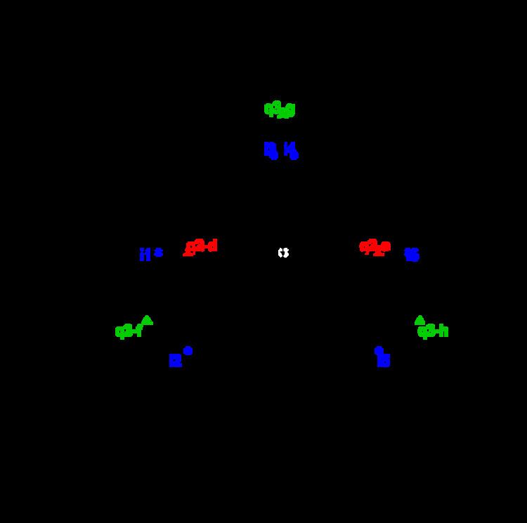
Six individuals ( i 1 , … , i 6 ) are described by three variables ( q 1 , q 2 , q 3 ) having respectively 3, 2 and 3 categories. Example : the individual i 1 possesses the category a of q 1 , d of q 2 and f of q 3 .

Applied to these data, the MCA function included in the R Package FactoMineR provides to the classical graph in Figure 1.

The relationship square (Figure 2) makes easier the reading of the classic factorial plane. It indicates that:

The first factor is related to the three variables but especially q 3 (which have a very high coordinate along the first axis) and then q 2 .

The second factor is related only to q 1 and q 3 (and not to q 2 which has a coordinate along axis 2 equal to 0) and that in a strong and equal manner.

All this is visible on the classic graphic but not so clearly. The role of the relationship square is first to assist in reading a conventional graphic. This is precious when the variables are numerous and possess numerous coordinates.

Extensions

This representation may be supplemented with those of quantitative variables, the coordinates of the latter being the square of correlation coefficients (and not of correlation ratios). Thus, the second advantage of the relationship square lies in the ability to represent simultaneously quantitative and qualitative variables.

The relationship square can be constructed from any factorial analysis of a table individuals x variables. In particular, it is (or should be) used systematically:

in multiple correspondences analysis (MCA);

in principal components analysis (PCA) when there are many supplementary variables;

in factor analysis of mixed data (FAMD).

An extension of this graphic to groups of variables (how to represent a group of variables by a single point ?) is used in Multiple Factor Analysis (MFA)

History

The idea of representing the qualitative variables themselves by a point (and not the categories) is due to Brigitte Escofier. The graphic as it is used now has been introduced by Brigitte Escofier and Jérôme Pagès in the framework of multiple factor analysis

Conclusion

In MCA, the relationship square provides a synthetic view of the connections between mixed variables, all the more valuable as there are many variables having many categories.This representation iscan be useful in any factorial analysis when there are numerous mixed variables, active and/or supplementary.

References

Relationship square Wikipedia

(Text) CC BY-SA