
 | ||
Real gases are non-hypothetical gases whose molecules occupy space and have interactions; consequently, they adhere to gas laws. To understand the behaviour of real gases, the following must be taken into account:
Contents
- Van der Waals model
- RedlichKwong model
- Berthelot and modified Berthelot model
- Dieterici model
- Clausius model
- Virial model
- PengRobinson model
- Wohl model
- BenedictWebbRubin model
- References
For most applications, such a detailed analysis is unnecessary, and the ideal gas approximation can be used with reasonable accuracy. On the other hand, real-gas models have to be used near the condensation point of gases, near critical points, at very high pressures, to explain the Joule–Thomson effect and in other less usual cases. The deviation from ideality can be described by the compressibility factor Z.
Van der Waals model
Real gases are often modeled by taking into account their molar weight and molar volume
or alternatively:
Where p is the pressure, T is the temperature, R the ideal gas constant, and Vm the molar volume. a and b are parameters that are determined empirically for each gas, but are sometimes estimated from their critical temperature (Tc) and critical pressure (pc) using these relations:
With the reduced properties
Redlich–Kwong model
The Redlich–Kwong equation is another two-parameter equation that is used to model real gases. It is almost always more accurate than the van der Waals equation, and often more accurate than some equations with more than two parameters. The equation is
or alternatively:
where a and b two empirical parameters that are not the same parameters as in the van der Waals equation. These parameters can be determined:
Using
Berthelot and modified Berthelot model
The Berthelot equation (named after D. Berthelot) is very rarely used,
but the modified version is somewhat more accurate
Dieterici model
This model (named after C. Dieterici) fell out of usage in recent years
with parameters a,b and
Clausius model
The Clausius equation (named after Rudolf Clausius) is a very simple three-parameter equation used to model gases.
or alternatively:
where
where Vc is critical volume.
Virial model
The Virial equation derives from a perturbative treatment of statistical mechanics.
or alternatively
where A, B, C, A′, B′, and C′ are temperature dependent constants.
Peng–Robinson model
Peng–Robinson equation of state (named after D.-Y. Peng and D. B. Robinson) has the interesting property being useful in modeling some liquids as well as real gases.
Wohl model
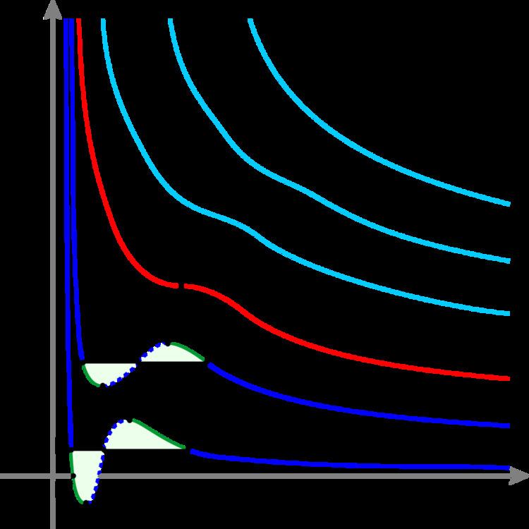
The Wohl equation (named after A. Wohl) is formulated in terms of critical values, making it useful when real gas constants are not available, but it cannot be used for high densities, as for example the critical isotherm shows a drastic decrease of pressure when the volume is contracted beyond the critical volume.
or:
or alternatively:
where
And with the reduced properties
This equation is based on five experimentally determined constants. It is expressed as
where
This equation is known to be reasonably accurate for densities up to about 0.8 ρcr, where ρcr is the density of the substance at its critical point. The constants appearing in the above equation are available in following table when p is in kPa, v is in
Benedict–Webb–Rubin model
The BWR equation, sometimes referred to as the BWRS equation,
where d is the molar density and where a, b, c, A, B, C, α, and γ are empirical constants. Note that the γ constant is a derivative of constant α and therefore almost identical to 1.