
 | ||
The Rankine–Hugoniot conditions, also referred to as Rankine–Hugoniot jump conditions or Rankine–Hugoniot relations, describe the relationship between the states on both sides of a shock wave in a one-dimensional flow in fluids or a one-dimensional deformation in solids. They are named in recognition of the work carried out by Scottish engineer and physicist William John Macquorn Rankine and French engineer Pierre Henri Hugoniot. See also Salas (2006) for some historical background.
Contents
- Basics Euler equations in one dimension
- The jump condition
- Euler equations shock condition
- Stationary shock
- Shock Hugoniot and Rayleigh line in solids
- Hugoniot elastic limit
- References
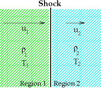
In a coordinate system that is moving with the shock, the Rankine–Hugoniot conditions can be expressed as:
where us is the shock wave speed, ρ1 and ρ2 are the mass density of the fluid behind and inside the shock, u2 is the particle velocity of the fluid inside the shock, p1 and p2 are the pressures in the two regions, and e1 and e2 are the specific (with the sense of per unit mass) internal energies in the two regions. These equations can be derived in a straightforward manner from equations (12), (13) and (14) below. Using the Rankine-Hugoniot equations for the conservation of mass and momentum to eliminate us and u2, the equation for the conservation of energy can be expressed as the Hugoniot equation:
where v1 and v2 are the uncompressed and compressed specific volumes per unit mass, respectively.
Basics: Euler equations in one dimension
Consider gas in a one-dimensional container (e.g., a long thin tube). Assume that the fluid is inviscid (i.e., it shows no viscosity effects as for example friction with the tube walls). Furthermore, assume that there is no heat transfer by conduction or radiation and that gravitational acceleration can be neglected. Such a system can be described by the following system of conservation laws, known as the 1D Euler equations, that in conservation form is:
where
Assume further that the gas is calorically ideal and that therefore a polytropic equation-of-state of the simple form
is valid, where
For an extensive list of compressible flow equations, etc., refer to NACA Report 1135 (1953).
Note: For a calorically ideal gas
The jump condition
Before proceeding further it is necessary to introduce the concept of a jump condition – a condition that holds at a discontinuity or abrupt change.
Consider a 1D situation where there is a jump in the scalar conserved physical quantity
for any
for smooth solutions.
Let the solution exhibit a jump (or shock) at
The subscripts 1 and 2 indicate conditions just upstream and just downstream of the jump respectively, i.e.
Note, to arrive at equation (8) we have used the fact that
Now, let
where we have defined
Equation (9) represents the jump condition for conservation law (6). A shock situation arises in a system where its characteristics intersect, and under these conditions a requirement for a unique single-valued solution is that the solution should satisfy the admissibility condition or entropy condition. For physically real applications this means that the solution should satisfy the Lax entropy condition
where
Euler equations shock condition
In the case of the hyperbolic conservation law (6), we have seen that the shock speed can be obtained by simple division. However, for the 1D Euler equations ( 1), ( 2) and ( 3), we have the vector state variable
Equations (12), (13) and (14) are known as the Rankine–Hugoniot conditions for the Euler equations and are derived by enforcing the conservation laws in integral form over a control volume that includes the shock. For this situation
where
See Laney (1998), LeVeque (2002), Toro (1999), Wesseling (2001), and Whitham (1999) for further discussion.
Stationary shock
For a stationary shock
In view of equation (16) we can simplify equation (18) to
which is a statement of Bernoulli's principle, under conditions where gravitational effects can be neglected.
Substituting
where
From physical considerations it is clear that both the upstream and downstream pressures must be positive, and this imposes an upper limit on the density ratio in equations (21) and (22) such that
Shock Hugoniot and Rayleigh line in solids
For shocks in solids, a closed form expression such as equation (15) cannot be derived from first principles. Instead, experimental observations indicate that a linear relation can be used instead (called the shock Hugoniot in the us-up plane) that has the form
where c0 is the bulk speed of sound in the material (in uniaxial compression), s is a parameter (the slope of the shock Hugoniot) obtained from fits to experimental data, and up=u2 is the particle velocity inside the compressed region behind the shock front.
The above relation, when combined with the Hugoniot equations for the conservation of mass and momentum, can be used to determine the shock Hugoniot in the p-v plane, where v is the specific volume (per unit mass):
Alternative equations of state, such as the Mie–Gruneisen equation of state may also be used instead of the above equation.
The shock Hugoniot describes the locus of all possible thermodynamic states a material can exist in behind a shock, projected onto a two dimensional state-state plane. It is therefore a set of equilibrium states and does not specifically represent the path through which a material undergoes transformation.
Weak shocks are isentropic and that the isentrope represents the path through which the material is loaded from the initial to final states by a compression wave with converging characteristics. In the case of weak shocks, the Hugoniot will therefore fall directly on the isentrope and can be used directly as the equivalent path. In the case of a strong shock we can no longer make that simplification directly. However, for engineering calculations, it is deemed that the isentrope is close enough to the Hugoniot that the same assumption can be made.
If the Hugoniot is approximately the loading path between states for an "equivalent" compression wave, then the jump conditions for the shock loading path can be determined by drawing a straight line between the initial and final states. This line is called the Rayleigh line and has the following equation:
Hugoniot elastic limit
Most solid materials undergo plastic deformations when subjected to strong shocks. The point on the shock Hugoniot at which a material transitions from a purely elastic state to an elastic-plastic state is called the Hugoniot elastic limit (HEL) and the pressure at which this transition takes place is denoted pHEL. Values of pHEL can range from 0.2 GPa to 20 GPa. Above the HEL, the material loses much of its shear strength and starts behaving like a fluid.