
 | ||
Randomized (Block) Coordinate Descent Method is an optimization algorithm popularized by Nesterov (2010) and Richtárik and Takáč (2011). The first analysis of this method, when applied to the problem of minimizing a smooth convex function, was performed by Nesterov (2010). In Nesterov's analysis the method needs to be applied to a quadratic perturbation of the original function with an unknown scaling factor. Richtárik and Takáč (2011) give iteration complexity bounds which do not require this, i.e., the method is applied to the objective function directly. Furthermore, they generalize the setting to the problem of minimizing a composite function, i.e., sum of a smooth convex and a (possibly nonsmooth) convex block-separable function:
Contents
- Algorithm
- Convergence rate
- Example on particular function
- Extension to Block Coordinate Setting
- References
where
Example (block decomposition): If
Example (block-separable regularizers):
-
n = N ; Ψ ( x ) = ∥ x ∥ 1 = ∑ i = 1 n | x i | -
N = N 1 + N 2 + ⋯ + N n ; Ψ ( x ) = ∑ i = 1 n ∥ x ( i ) ∥ 2 x ( i ) ∈ R N i ∥ ⋅ ∥ 2
Algorithm
Consider the optimization problem
where
Smoothness: By smoothness we mean the following: we assume the gradient of
for all
Nesterov, and Richtarik and Takac showed that the following algorithm converges to the optimal point:
Convergence rate
Since the iterates of this algorithm are random vectors, a complexity result would give a bound on the number of iterations needed for the method to output an approximate solution with high probability. It was shown in that if
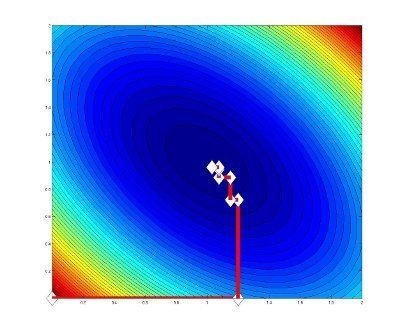
Example on particular function
The following Figure shows how
Extension to Block Coordinate Setting
One can naturally extend this algorithm not only just to coordinates, but to blocks of coordinates. Assume that we have space