
 | ||
The rainflow-counting algorithm (also known as the "rain-flow counting method") is used in the analysis of fatigue data in order to reduce a spectrum of varying stress into a set of simple stress reversals. Its importance is that it allows the application of Miner's rule in order to assess the fatigue life of a structure subject to complex loading. The algorithm was developed by Tatsuo Endo and M. Matsuishi in 1968. Though there are a number of cycle-counting algorithms for such applications, the rainflow method is the most popular as of 2008.
Contents
Downing and Socie created one of the more widely referenced and utilized rainflow cycle-counting algorithms in 1982, which was included as one of many cycle-counting algorithms in ASTM E 1049-85. This algorithm is used in Sandia National Laboratories LIFE2 code for the fatigue analysis of wind turbine components.
Igor Rychlik gave a mathematical definition for the rainflow counting method, thus enabling closed-form computations from the statistical properties of the load signal.
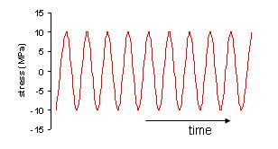
For simple periodic loadings, such as Figure 1, rainflow counting is unnecessary. That sequence clearly has 10 cycles of amplitude 10 MPa and a structure's life can be estimated from a simple application of the relevant S-N curve.
Compare this with Figure 2 which cannot be assessed in terms of simply-described stress reversals.
Algorithm
- Reduce the time history to a sequence of (tensile) peaks and (compressive) valleys.
- Imagine that the time history is a template for a rigid sheet (pagoda roof).
- Turn the sheet clockwise 90° (earliest time to the top).
- Each tensile peak is imagined as a source of water that "drips" down the pagoda.
- Count the number of half-cycles by looking for terminations in the flow occurring when either:
- It reaches the end of the time history;
- It merges with a flow that started at an earlier tensile peak; or
- It flows when an opposite tensile peak has greater magnitude.
- Repeat step 5 for compressive valleys.
- Assign a magnitude to each half-cycle equal to the stress difference between its start and termination.
- Pair up half-cycles of identical magnitude (but opposite sense) to count the number of complete cycles. Typically, there are some residual half-cycles.
Example
Block Loading example
There are many cases in which a structure will undergo periodic loading. Assume that a specimen is loaded periodically until failure. The number of blocks endured before failure can be determined easily by using the Palmgren-Miner rule of block loading. The actual load history is shown in Figure 5.
If all of the similar loads are grouped together, it forms a series of block loads as shown in Figure 6.
The Palmgren-Miner rule can be expressed as
where,
B = number of blocksNk = number of cycles of loading condition, kNfk =number of cycles to failure for loading condition, kIn this example, each Nk=1 because there is one instance of each load for every period of loading. To find Nf (number of loads to failure) for each load the Goodman-Basquin relation can be used
where,
σa = stress amplitudeσ'f = fatigue strength coefficient (material property)σm = mean stressσult = ultimate stress (material property)b = fatigue strength exponent (material property)Assumptions
There are two key assumptions made in order to rearrange the loads into blocks. These assumptions may affect the validity of the procedure depending on the situation.