Quasi Monte Carlo methods in finance

Monte Carlo and quasi-Monte Carlo methods

Integrals in hundreds or thousands of variables are common in computational finance. These have to be approximated numerically to within an error threshold ϵ . It is well known that if a worst case guarantee of error at most ϵ is required then the computational complexity of integration may be exponential in d , the dimension of the integrand; See Ch. 3 for details. To break this curse of dimensionality one can use the Monte Carlo (MC) method defined by

where the evaluation points x i are randomly chosen. It is well known that the expected error of Monte Carlo is of order n − 1 / 2 . Thus the cost of the algorithm that has error ϵ is of order ϵ − 2 breaking the curse of dimensionality.

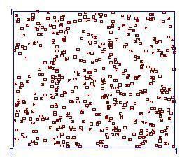
Of course in computational practice pseudo-random points are used. Figure 1 shows the distribution of 500 pseudo-random points on the unit square.

Note there are regions where there are no points and other regions where there are clusters of points. It would be desirable to sample the integrand at uniformly distributed points. A rectangular grid would be uniform but even if there were only 2 grid points in each Cartesian direction there would be 2 d points. So the desideratum should be as few points as possible chosen as uniform as possible.

It turns out there is a well-developed part of number theory which deals exactly with this desideratum. Discrepancy is a measure of deviation from uniformity so what one wants are low discrepancy sequences (LDS). Numerous LDS have been created named after their inventors, e.g.

Figure 2. gives the distribution of 500 LDS points.

The quasi-Monte Carlo (QMC) method is defined by

where the x i belong to an LDS. The standard terminology quasi-Monte Carlo is somewhat unfortunate since MC is a randomized method whereas QMC is purely deterministic.

The uniform distribution of LDS is desirable. But the worst case error of QMC is of order

where n is the number of sample points. See for the theory of LDS and references to the literature. The rate of convergence of LDS may be contrasted with the expected rate of convergence of MC which is n − 1 / 2 . For d small the rate of convergence of QMC is faster than MC but for d large the factor ( log ⁡ n ) d is devastating. For example, if d = 360 , then even with log ⁡ n = 2 the QMC error is proportional to 2 360 . Thus it was widely believed by the world's leading experts that QMC should not be used for high-dimensional integration. For example, in 1992 Bratley, Fox and Niederreiter performed extensive testing on certain mathematical problems. They conclude "in high-dimensional problems (say d > 12 ), QMC seems to offer no practical advantage over MC". In 1993, Rensburg and Torrie compared QMC with MC for the numerical estimation of high-dimensional integrals which occur in computing virial coefficients for the hard-sphere fluid. They conclude QMC is more effective than MC only if d < 10 . As we shall see, tests on 360-dimensional integrals arising from a collateralized mortgage obligation (CMO) lead to very different conclusions.

Woźniakowski's 1991 paper showing the connection between average case complexity of integration and QMC led to new interest in QMC. Woźniakowski's result received considerable coverage in the scientific press . In early 1992, I. T. Vanderhoof, New York University, became aware of Woźniakowski's result and gave Woźniakowski's colleague J. F. Traub, Columbia University, a CMO with parameters set by Goldman Sachs. This CMO had 10 tranches each requiring the computation of a 360 dimensional integral. Traub asked a Ph.D. student, Spassimir Paskov, to compare QMC with MC for the CMO. In 1992 Paskov built a software system called FinDer and ran extensive tests. To the Columbia's research group's surprise and initial disbelief Paskov reported that QMC was always superior to MC in a number of ways. Details are given below. Preliminary results were presented by Paskov and Traub to a number of Wall Street firms in Fall 1993 and Spring 1994. The firms were initially skeptical of the claim that QMC was superior to MC for pricing financial derivatives. A January 1994 article in Scientific American by Traub and Woźniakowski discussed the theoretical issues and reported that "Preliminary results obtained by testing certain finance problems suggests the superiority of the deterministic methods in practice". In Fall 1994 Paskov wrote a Columbia University Computer Science Report which appeared in slightly modified form in 1997.

In Fall 1995 Paskov and Traub published a paper in the "Journal of Portfolio Management". They compared MC and two QMC methods. The two deterministic methods used Sobol and Halton points. Since better LDS were created later, no comparison will be made between Sobol and Halton sequences. The experiments drew the following conclusions regarding the performance of MC and QMC on the 10 tranche CMO:

To summarize, QMC beats MC for the CMO on accuracy, confidence level, and speed.

This paper was followed by reports on tests by a number of researchers which also led to the conclusion the QMC is superior to MC for a variety of high-dimensional finance problems. This includes papers by Caflisch and Morokoff (1996), Joy, Boyle, Tan (1996), Ninomiya and Tezuka (1996), Papageorgiou and Traub (1996), Ackworth, Broadie and Glasserman (1997), Kucherenko and co-authors

Further testing of the CMO was carried out by Anargyros Papageorgiou, who developed an improved version of the FinDer software system. The new results include the following:

Currently the highest reported dimension for which QMC outperforms MC is 65536. The software is the Sobol' Sequence generator SobolSeq65536 which generates Sobol' Sequences satisfying Property A for all dimensions and Property A' for the adjacent dimensions. SobolSeq generators outperform all other known generators both in speed and accuracy

Theoretical explanations

The results reported so far in this article are empirical. A number of possible theoretical explanations have been advanced. This has been a very research rich area leading to powerful new concepts but a definite answer has not been obtained.

A possible explanation of why QMC is good for finance is the following. Consider a tranche of the CMO mentioned earlier. The integral gives expected future cash flows from a basket of 30-year mortgages at 360 monthly intervals. Because of the discounted value of money variables representing future times are increasingly less important. In a seminal paper I. Sloan and H. Woźniakowski introduced the idea of weighted spaces. In these spaces the dependence on the successive variables can be moderated by weights. If the weights decrease sufficiently rapidly the curse of dimensionality is broken even with a worst case guarantee. This paper led to a great amount of work on the tractability of integration and other problems. A problem is tractable when its complexity is of order ϵ − p and p is independent of the dimension.

On the other hand, effective dimension was proposed by Caflisch, Morokoff and Owen as an indicator of the difficulty of high-dimensional integration. The purpose was to explain the remarkable success of quasi-Monte Carlo (QMC) in approximating the very-high-dimensional integrals in finance. They argued that the integrands are of low effective dimension and that is why QMC is much faster than Monte Carlo (MC). The impact of the arguments of Caflisch et al. was great. A number of papers deal with the relationship between the error of QMC and the effective dimension .

It is known that QMC fails for certain functions that have high effective dimension. However, low effective dimension is not a necessary condition for QMC to beat MC and for high-dimensional integration to be tractable. In 2005, Tezuka exhibited a class of functions of d variables, all with maximum effective dimension equal to d . For these functions QMC is very fast since its convergence rate is of order n − 1 , where n is the number of function evaluations.

Isotropic integrals

QMC can also be superior to MC and to other methods for isotropic problems, that is, problems where all variables are equally important. For example, Papageorgiou and Traub reported test results on the model integration problems suggested by the physicist B. D. Keister

where ∥ ⋅ ∥ denotes the Euclidean norm and d = 25 . Keister reports that using a standard numerical method some 220,000 points were needed to obtain a relative error on the order of 10 − 2 . A QMC calculation using the generalized Faure low discrepancy sequence (QMC-GF) used only 500 points to obtain the same relative error. The same integral was tested for a range of values of d up to d = 100 . Its error was

c < 110 , where n is the number of evaluations of f . This may be compared with the MC method whose error was proportional to n − 1 / 2 .

These are empirical results. In a theoretical investigation Papageorgiou proved that the convergence rate of QMC for a class of d -dimensional isotropic integrals which includes the integral defined above is of the order

This is with a worst case guarantee compared to the expected convergence rate of n − 1 / 2 of Monte Carlo and shows the superiority of QMC for this type of integral.

In another theoretical investigation Papageorgiou presented sufficient conditions for fast QMC convergence. The conditions apply to isotropic and non-isotropic problems and, in particular, to a number of problems in computational finance. He presented classes of functions where even in the worst case the convergence rate of QMC is of order

where p ≥ 0 is a constant that depends on the class of functions.

But this is only a sufficient condition and leaves open the major question we pose in the next section.

Open questions

1. Characterize for which high-dimensional integration problems QMC is superior to MC.
2. Characterize types of financial instruments for which QMC is superior to MC.