Quantum tunnelling

History

Quantum tunnelling was developed from the study of radioactivity, which was discovered in 1896 by Henri Becquerel. Radioactivity was examined further by Marie Curie and Pierre Curie, for which they earned the Nobel Prize in Physics in 1903. Ernest Rutherford and Egon Schweidler studied its nature, which was later verified empirically by Friedrich Kohlrausch. The idea of the half-life and the impossibility of predicting decay was created from their work.

In 1901, Robert Francis Earhart, while investigating the conduction of gases between closely spaced electrodes using the Michelson interferometer to measure the spacing, discovered an unexpected conduction regime. J. J. Thomson commented the finding warranted further investigation. In 1911 and then 1914, then-graduate student Franz Rother, employing Earhart's method for controlling and measuring the electrode separation but with a sensitive platform galvanometer, directly measured steady field emission currents. In 1926, Rother, using a still newer platform galvanometer of sensitivity 26 pA, measured the field emission currents in a "hard" vacuum between closely spaced electrodes.

Friedrich Hund was the first to take notice of tunnelling in 1927 when he was calculating the ground state of the double-well potential. Its first application was a mathematical explanation for alpha decay, which was done in 1928 by George Gamow and independently by Ronald Gurney and Edward Condon. The two researchers simultaneously solved the Schrödinger equation for a model nuclear potential and derived a relationship between the half-life of the particle and the energy of emission that depended directly on the mathematical probability of tunnelling.

After attending a seminar by Gamow, Max Born recognised the generality of tunnelling. He realised that it was not restricted to nuclear physics, but was a general result of quantum mechanics that applies to many different systems. Shortly thereafter, both groups considered the case of particles tunnelling into the nucleus. The study of semiconductors and the development of transistors and diodes led to the acceptance of electron tunnelling in solids by 1957. The work of Leo Esaki, Ivar Giaever and Brian Josephson predicted the tunnelling of superconducting Cooper pairs, for which they received the Nobel Prize in Physics in 1973. In 2016, the quantum tunneling of water was discovered.

Introduction to the concept

Quantum tunnelling falls under the domain of quantum mechanics: the study of what happens at the quantum scale. This process cannot be directly perceived, but much of its understanding is shaped by the microscopic world, which classical mechanics cannot adequately explain. To understand the phenomenon, particles attempting to travel between potential barriers can be compared to a ball trying to roll over a hill; quantum mechanics and classical mechanics differ in their treatment of this scenario. Classical mechanics predicts that particles that do not have enough energy to classically surmount a barrier will not be able to reach the other side. Thus, a ball without sufficient energy to surmount the hill would roll back down. Or, lacking the energy to penetrate a wall, it would bounce back (reflection) or in the extreme case, bury itself inside the wall (absorption). In quantum mechanics, these particles can, with a very small probability, tunnel to the other side, thus crossing the barrier. Here, the "ball" could, in a sense, borrow energy from its surroundings to tunnel through the wall or "roll over the hill", paying it back by making the reflected electrons more energetic than they otherwise would have been.

The reason for this difference comes from the treatment of matter in quantum mechanics as having properties of waves and particles. One interpretation of this duality involves the Heisenberg uncertainty principle, which defines a limit on how precisely the position and the momentum of a particle can be known at the same time. This implies that there are no solutions with a probability of exactly zero (or one), though a solution may approach infinity if, for example, the calculation for its position was taken as a probability of 1, the other, i.e. its speed, would have to be infinity. Hence, the probability of a given particle's existence on the opposite side of an intervening barrier is non-zero, and such particles will appear on the 'other' (a semantically difficult word in this instance) side with a relative frequency proportional to this probability.

The tunnelling problem

The wave function of a particle summarises everything that can be known about a physical system. Therefore, problems in quantum mechanics center on the analysis of the wave function for a system. Using mathematical formulations of quantum mechanics, such as the Schrödinger equation, the wave function can be solved. This is directly related to the probability density of the particle's position, which describes the probability that the particle is at any given place. In the limit of large barriers, the probability of tunnelling decreases for taller and wider barriers.

For simple tunnelling-barrier models, such as the rectangular barrier, an analytic solution exists. Problems in real life often do not have one, so "semiclassical" or "quasiclassical" methods have been developed to give approximate solutions to these problems, like the WKB approximation. Probabilities may be derived with arbitrary precision, constrained by computational resources, via Feynman's path integral method; such precision is seldom required in engineering practice.

Related phenomena

There are several phenomena that have the same behaviour as quantum tunnelling, and thus can be accurately described by tunnelling. Examples include the tunnelling of a classical wave-particle association, evanescent wave coupling (the application of Maxwell's wave-equation to light) and the application of the non-dispersive wave-equation from acoustics applied to "waves on strings". Evanescent wave coupling, until recently, was only called "tunnelling" in quantum mechanics; now it is used in other contexts.

These effects are modelled similarly to the rectangular potential barrier. In these cases, there is one transmission medium through which the wave propagates that is the same or nearly the same throughout, and a second medium through which the wave travels differently. This can be described as a thin region of medium B between two regions of medium A. The analysis of a rectangular barrier by means of the Schrödinger equation can be adapted to these other effects provided that the wave equation has travelling wave solutions in medium A but real exponential solutions in medium B.

In optics, medium A is a vacuum while medium B is glass. In acoustics, medium A may be a liquid or gas and medium B a solid. For both cases, medium A is a region of space where the particle's total energy is greater than its potential energy and medium B is the potential barrier. These have an incoming wave and resultant waves in both directions. There can be more mediums and barriers, and the barriers need not be discrete; approximations are useful in this case.

Applications

Tunnelling occurs with barriers of thickness around 1-3 nm and smaller, but is the cause of some important macroscopic physical phenomena. For instance, tunnelling is a source of current leakage in very-large-scale integration (VLSI) electronics and results in the substantial power drain and heating effects that plague high-speed and mobile technology; it is considered the lower limit on how small computer chips can be made. Tunnelling is a fundamental technique used to program the floating gates of FLASH memory, which is one of the most significant inventions that have shaped consumer electronics in the last two decades.

Nuclear fusion in stars

Quantum tunnelling is essential for nuclear fusion in stars. Temperature and pressure in the core of stars are insufficient for nuclei to overcome the Coulomb barrier in order to achieve a thermonuclear fusion. However, there is some probability to penetrate the barrier due to quantum tunnelling. Though the probability is very low, the extreme number of nuclei in a star generates a steady fusion reaction over millions or even billions of years - a precondition for the evolution of life in insolation habitable zones.

Radioactive decay

Radioactive decay is the process of emission of particles and energy from the unstable nucleus of an atom to form a stable product. This is done via the tunnelling of a particle out of the nucleus (an electron tunnelling into the nucleus is electron capture). This was the first application of quantum tunnelling and led to the first approximations. Radioactive decay is also a relevant issue for astrobiology as this consequence of quantum tunnelling is creating a constant source of energy over a large period of time for environments outside the circumstellar habitable zone where insolation would not be possible (subsurface oceans) or effective.

Astrochemistry in interstellar clouds

By including quantum tunnelling the astrochemical syntheses of various molecules in interstellar clouds can be explained such as the synthesis of molecular hydrogen, water (ice) and the prebiotic important Formaldehyde.

Quantum biology

Quantum tunnelling is among the central non trivial quantum effects in quantum biology. Here it is important both as electron tunnelling and proton tunnelling. Electron tunnelling is a key factor in many biochemical redox reactions (photosynthesis, cellular respiration) as well as enzymatic catalysis while proton tunnelling is a key factor in spontaneous mutation of DNA.

Spontaneous mutation of DNA occurs when normal DNA replication takes place after a particularly significant proton has defied the odds in quantum tunnelling in what is called "proton tunnelling" (quantum biology). A hydrogen bond joins normal base pairs of DNA. There exists a double well potential along a hydrogen bond separated by a potential energy barrier. It is believed that the double well potential is asymmetric with one well deeper than the other so the proton normally rests in the deeper well. For a mutation to occur, the proton must have tunnelled into the shallower of the two potential wells. The movement of the proton from its regular position is called a tautomeric transition. If DNA replication takes place in this state, the base pairing rule for DNA may be jeopardised causing a mutation. Per-Olov Lowdin was the first to develop this theory of spontaneous mutation within the double helix (quantum bio). Other instances of quantum tunnelling-induced mutations in biology are believed to be a cause of ageing and cancer.

Cold emission

Cold emission of electrons is relevant to semiconductors and superconductor physics. It is similar to thermionic emission, where electrons randomly jump from the surface of a metal to follow a voltage bias because they statistically end up with more energy than the barrier, through random collisions with other particles. When the electric field is very large, the barrier becomes thin enough for electrons to tunnel out of the atomic state, leading to a current that varies approximately exponentially with the electric field. These materials are important for flash memory, vacuum tubes, as well as some electron microscopes.

Tunnel junction

A simple barrier can be created by separating two conductors with a very thin insulator. These are tunnel junctions, the study of which requires quantum tunnelling. Josephson junctions take advantage of quantum tunnelling and the superconductivity of some semiconductors to create the Josephson effect. This has applications in precision measurements of voltages and magnetic fields, as well as the multijunction solar cell.

Tunnel diode

Diodes are electrical semiconductor devices that allow electric current flow in one direction more than the other. The device depends on a depletion layer between N-type and P-type semiconductors to serve its purpose; when these are very heavily doped the depletion layer can be thin enough for tunnelling. Then, when a small forward bias is applied the current due to tunnelling is significant. This has a maximum at the point where the voltage bias is such that the energy level of the p and n conduction bands are the same. As the voltage bias is increased, the two conduction bands no longer line up and the diode acts typically.

Because the tunnelling current drops off rapidly, tunnel diodes can be created that have a range of voltages for which current decreases as voltage is increased. This peculiar property is used in some applications, like high speed devices where the characteristic tunnelling probability changes as rapidly as the bias voltage.

The resonant tunnelling diode makes use of quantum tunnelling in a very different manner to achieve a similar result. This diode has a resonant voltage for which there is a lot of current that favors a particular voltage, achieved by placing two very thin layers with a high energy conductance band very near each other. This creates a quantum potential well that have a discrete lowest energy level. When this energy level is higher than that of the electrons, no tunnelling will occur, and the diode is in reverse bias. Once the two voltage energies align, the electrons flow like an open wire. As the voltage is increased further tunnelling becomes improbable and the diode acts like a normal diode again before a second energy level becomes noticeable.

Tunnel field-effect transistors

A European research project has demonstrated field effect transistors in which the gate (channel) is controlled via quantum tunnelling rather than by thermal injection, reducing gate voltage from ~1 volt to 0.2 volts and reducing power consumption by up to 100×. If these transistors can be scaled up into VLSI chips, they will significantly improve the performance per power of integrated circuits.

Quantum conductivity

While the Drude model of electrical conductivity makes excellent predictions about the nature of electrons conducting in metals, it can be furthered by using quantum tunnelling to explain the nature of the electron's collisions. When a free electron wave packet encounters a long array of uniformly spaced barriers the reflected part of the wave packet interferes uniformly with the transmitted one between all barriers so that there are cases of 100% transmission. The theory predicts that if positively charged nuclei form a perfectly rectangular array, electrons will tunnel through the metal as free electrons, leading to an extremely high conductance, and that impurities in the metal will disrupt it significantly.

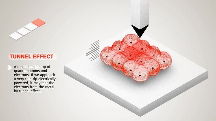
Scanning tunnelling microscope

The scanning tunnelling microscope (STM), invented by Gerd Binnig and Heinrich Rohrer, allows imaging of individual atoms on the surface of a metal. It operates by taking advantage of the relationship between quantum tunnelling with distance. When the tip of the STM's needle is brought very close to a conduction surface that has a voltage bias, by measuring the current of electrons that are tunnelling between the needle and the surface, the distance between the needle and the surface can be measured. By using piezoelectric rods that change in size when voltage is applied over them the height of the tip can be adjusted to keep the tunnelling current constant. The time-varying voltages that are applied to these rods can be recorded and used to image the surface of the conductor. STMs are accurate to 0.001 nm, or about 1% of atomic diameter.

Faster than light

It is possible for spin zero particles to travel faster than the speed of light when tunnelling. This apparently violates the principle of causality, since there will be a frame of reference in which it arrives before it has left. However, careful analysis of the transmission of the wave packet shows that there is actually no violation of relativity theory. In 1998, Francis E. Low reviewed briefly the phenomenon of zero time tunnelling. More recently experimental tunnelling time data of phonons, photons, and electrons have been published by Günter Nimtz.

Mathematical discussions of quantum tunnelling

The following subsections discuss the mathematical formulations of quantum tunnelling.

The Schrödinger equation

The time-independent Schrödinger equation for one particle in one dimension can be written as

− ℏ 2 2 m d 2 d x 2 Ψ ( x ) + V ( x ) Ψ ( x ) = E Ψ ( x ) or d 2 d x 2 Ψ ( x ) = 2 m ℏ 2 ( V ( x ) − E ) Ψ ( x ) ≡ 2 m ℏ 2 M ( x ) Ψ ( x ) ,

where ℏ is the reduced Planck's constant, m is the particle mass, x represents distance measured in the direction of motion of the particle, Ψ is the Schrödinger wave function, V is the potential energy of the particle (measured relative to any convenient reference level), E is the energy of the particle that is associated with motion in the x-axis (measured relative to V), and M(x) is a quantity defined by V(x) – E which has no accepted name in physics.

The solutions of the Schrödinger equation take different forms for different values of x, depending on whether M(x) is positive or negative. When M(x) is constant and negative, then the Schrödinger equation can be written in the form

d 2 d x 2 Ψ ( x ) = 2 m ℏ 2 M ( x ) Ψ ( x ) = − k 2 Ψ ( x ) , w h e r e k 2 = − 2 m ℏ 2 M .

The solutions of this equation represent traveling waves, with phase-constant +k or -k. Alternatively, if M(x) is constant and positive, then the Schrödinger equation can be written in the form

d 2 d x 2 Ψ ( x ) = 2 m ℏ 2 M ( x ) Ψ ( x ) = κ 2 Ψ ( x ) , w h e r e κ 2 = 2 m ℏ 2 M .

The solutions of this equation are rising and falling exponentials in the form of evanescent waves. When M(x) varies with position, the same difference in behaviour occurs, depending on whether M(x) is negative or positive. It follows that the sign of M(x) determines the nature of the medium, with negative M(x) corresponding to medium A as described above and positive M(x) corresponding to medium B. It thus follows that evanescent wave coupling can occur if a region of positive M(x) is sandwiched between two regions of negative M(x), hence creating a potential barrier.

The mathematics of dealing with the situation where M(x) varies with x is difficult, except in special cases that usually do not correspond to physical reality. A discussion of the semi-classical approximate method, as found in physics textbooks, is given in the next section. A full and complicated mathematical treatment appears in the 1965 monograph by Fröman and Fröman noted below. Their ideas have not been incorporated into physics textbooks, but their corrections have little quantitative effect.

The WKB approximation

The wave function is expressed as the exponential of a function:

Ψ ( x ) = e Φ ( x ) , where Φ ″ ( x ) + Φ ′ ( x ) 2 = 2 m ℏ 2 ( V ( x ) − E ) .

Φ ′ ( x ) is then separated into real and imaginary parts:

Φ ′ ( x ) = A ( x ) + i B ( x ) , where A(x) and B(x) are real-valued functions.

Substituting the second equation into the first and using the fact that the imaginary part needs to be 0 results in:

A ′ ( x ) + A ( x ) 2 − B ( x ) 2 = 2 m ℏ 2 ( V ( x ) − E ) .

To solve this equation using the semiclassical approximation, each function must be expanded as a power series in ℏ . From the equations, the power series must start with at least an order of ℏ − 1 to satisfy the real part of the equation; for a good classical limit starting with the highest power of Planck's constant possible is preferable, which leads to

A ( x ) = 1 ℏ ∑ k = 0 ∞ ℏ k A k ( x )

and

B ( x ) = 1 ℏ ∑ k = 0 ∞ ℏ k B k ( x ) ,

with the following constraints on the lowest order terms,

A 0 ( x ) 2 − B 0 ( x ) 2 = 2 m ( V ( x ) − E )

and

A 0 ( x ) B 0 ( x ) = 0 .

At this point two extreme cases can be considered.

Case 1 If the amplitude varies slowly as compared to the phase A 0 ( x ) = 0 and

which corresponds to classical motion. Resolving the next order of expansion yields

Case 2

If the phase varies slowly as compared to the amplitude, B 0 ( x ) = 0 and which corresponds to tunnelling. Resolving the next order of the expansion yields

In both cases it is apparent from the denominator that both these approximate solutions are bad near the classical turning points E = V ( x ) . Away from the potential hill, the particle acts similar to a free and oscillating wave; beneath the potential hill, the particle undergoes exponential changes in amplitude. By considering the behaviour at these limits and classical turning points a global solution can be made.

To start, choose a classical turning point, x 1 and expand 2 m ℏ 2 ( V ( x ) − E ) in a power series about x 1 :

2 m ℏ 2 ( V ( x ) − E ) = v 1 ( x − x 1 ) + v 2 ( x − x 1 ) 2 + ⋯

Keeping only the first order term ensures linearity:

2 m ℏ 2 ( V ( x ) − E ) = v 1 ( x − x 1 ) .

Using this approximation, the equation near x 1 becomes a differential equation:

d 2 d x 2 Ψ ( x ) = v 1 ( x − x 1 ) Ψ ( x ) .

This can be solved using Airy functions as solutions.

Ψ ( x ) = C A A i ( v 1 3 ( x − x 1 ) ) + C B B i ( v 1 3 ( x − x 1 ) )

Taking these solutions for all classical turning points, a global solution can be formed that links the limiting solutions. Given the 2 coefficients on one side of a classical turning point, the 2 coefficients on the other side of a classical turning point can be determined by using this local solution to connect them.

Hence, the Airy function solutions will asymptote into sine, cosine and exponential functions in the proper limits. The relationships between C , θ and C + , C − are

C + = 1 2 C cos ⁡ ( θ − π 4 )

and

C − = − C sin ⁡ ( θ − π 4 )

With the coefficients found, the global solution can be found. Therefore, the transmission coefficient for a particle tunnelling through a single potential barrier is

T ( E ) = e − 2 ∫ x 1 x 2 d x 2 m ℏ 2 [ V ( x ) − E ] ,

where x 1 , x 2 are the 2 classical turning points for the potential barrier.

For a rectangular barrier, this expression is simplified to:

T ( E ) = e − 2 2 m ℏ 2 ( V 0 − E ) ( x 2 − x 1 ) = V ~ 0 − ( x 2 − x 1 ) .