Preisach model of hysteresis

Nonideal relay

The relay hysteron is the fundamental building block of the Preisach model. It is described as a two-valued operator denoted by R α , β . Its I/O map takes the form of a loop, as shown:

Above, a relay of magnitude 1. α defines the "switch-off" threshold, and β defines the "switch-on" threshold.

Graphically, if x is less than α , the output y is "low" or "off." As we increase x , the output remains low until x reaches β —at which point the output switches "on." Further increasing x has no change. Decreasing x , y does not go low until x reaches α again. It is apparent that the relay operator R α , β takes the path of a loop, and its next state depends on its past state.

Mathematically, the output of R α , β is expressed as:

y ( x ) = { 1  if  x ≥ β 0  if  x ≤ α k  if  α < x < β

Where k = 0 if the last time x was outside of the boundaries α < x < β , it was in the region of x ≤ α ; and k = 1 if the last time x was outside of the boundaries α < x < β , it was in the region of x ≥ β .

This definition of the hysteron shows that the current value y of the complete hysteresis loop depends upon the history of the input variable x .

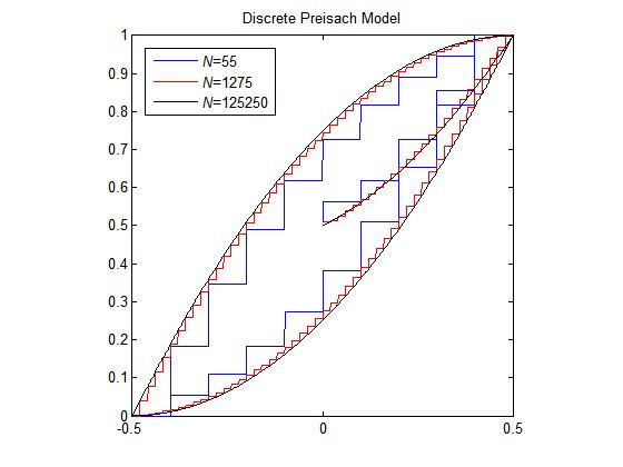
Discrete Preisach model

The Preisach model consists of many relay hysterons connected in parallel, given weights, and summed. This is best visualized by a block diagram:

Each of these relays has different α and β thresholds and is scaled by μ . Each relay can be plotted on a so-called Preisach plane with its ( α , β ) values. Depending on their distribution on the Preisach plane, the relay hysterons can represent hysteresis with good accuracy. As well, with increasing N , the true hysteresis curve is approximated better.

In the limit as N approaches infinity, we obtain the continuous Preisach model.

The α β {\displaystyle \alpha \beta } plane

One of the easiest ways to look at the Preisach model is using a geometric interpretation. Consider a plane of coordinates α β . On this plane, each point ( α i , β i ) is mapped to a specific relay hysteron R α i , β i .

We consider only the half-plane α < β as any other case does not have a physical equivalent in nature.

Next, we take a specific point on the half plane and build a right triangle by drawing two lines parallel to the axes, both from the point to the line α = β .

We now present the Preisach density function, denoted μ ( α , β ) . This function describes the amount of relay hysterons of each distinct values of ( α i , β i ) . As a default we say that outside the right triangle μ ( α , β ) = 0 .

A modified formulation of the classical Preisach model has been presented, allowing analytical expression of the Everett function. This makes the model considerably faster and especially adequate for inclusion in electromagnetic field computation or electric circuit analysis codes.

Vector Preisach Model

The vector Preisach model is constructed as the linear superposition of scalar models. For considering the uniaxial anisotropy of the material, Everett functions are expanded by Fourier coefficients. In this case, the measured and simulated curves are in a very good agreement.