Power system simulation

Load flow calculation

The load-flow calculation is the most common network analysis tool for examining the undisturbed and disturbed network within the scope of operational and strategic planning.

Using network topology, transmission line parameters, transformer parameters, generator location and limits, and load location and compensation, the load-flow calculation can provide voltage magnitudes and angles for all nodes and loading of network components, such as cables and transformers. With this information, compliance to operating limitations such as those stipulated by voltage ranges and maximum loads, can be examined. This is, for example, important for determining the transmission capacity of underground cables, where the influence of cable bundling on the load capability of each cable has to be taken also into account.

Due to the ability to determine losses and reactive-power allocation, load-flow calculation also supports the planning engineer in the investigation of the most economical operation mode of the network.

When changing over from single and/or multi-phase infeed low-voltage meshed networks to isolated networks, load-flow calculation is essential for operational and economical reasons. Load-flow calculation is also the basis of all further network studies, such as motor start-up or investigation of scheduled or unscheduled outages of equipment within the outage simulation.

Especially when investigating motor start-up, the load-flow calculation results give helpful hints, for example, of whether the motor can be started in spite of the voltage drop caused by the start-up current.

Short circuit analysis

Short circuit analysis analyzes the power flow after a fault occurs in a power network. The faults may be three-phase short circuit, one-phase grounded, two-phase short circuit, two-phase grounded, one-phase break, two-phase break or complex faults. Results of such an analysis may help determine the following:

1. Magnitude of the fault current
2. Circuit breaker capacity
3. Rise in voltage in a single line due to ground fault
4. Residual voltage and relay settings
5. Interference due to power line.

Transient stability simulation

The goal of transient stability simulation of power systems is to analyse the stability of a power system in a from sub-second to several tens of seconds. Stability in this aspect is the ability of the system to quickly return to a stable operating condition after being exposed to a disturbance such as for example a tree falling over an overhead line resulting in the automatic disconnection of that line by its protection systems. In engineering terms, a power system is deemed stable if the substation voltage levels and the rotational speeds of motors and generators return to their normal values in a quick and continuous manner.

Models typically use the following inputs:

Number, size and type of generators with any available mechanical, electrical, and control (governor, voltage regulation, etc.) parameters,

a mix of residential, commercial and industrial load at each bus,

location and specifications for distributed control devices such as tap-changing transformers, switched shunt compensation, static Var compensators, flexible AC transmission systems, etc.,

location and specifications for protection devices such as relays and load shedding, and

location and specifications of any other relevant control and/or protection devices.

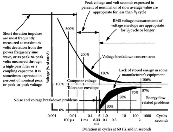
The acceptable amount of time it takes grid voltages return to their intended levels is dependent on the magnitude of voltage disturbance, and the most common standard is specified by the CBEMA curve in Figure. 1. This curve informs both electronic equipment design and grid stability data reporting.

Unit commitment

The problem of unit commitment involves finding the least-cost dispatch of available generation resources to meet the electrical load.

Generating resources can include a wide range of types:

1. Nuclear
2. Thermal (using coal, gas, other fossil fuels, or biomass)
3. Renewables (including hydro, wind, wave-power, and solar)

The key decision variables that are decided by the computer program are:

1. Generation level (in megawatts)
2. Number of generating units on

The latter decisions are binary {0,1}, which means that the mathematical problem is not continuous.

In addition, generating plants are subject to a number of complex technical constraints, including:

1. Minimum stable operating level
2. Maximum rate of ramping up or down
3. Minimum time period the unit is up and/or down

These constraints have many different variants; all this gives rise to a large class of mathematical optimization problems.

Optimal power flow

Electricity flows through an AC network according to Kirchhoff's Laws. Transmission lines are subject to thermal limits (simple megawatt limits on flow), as well as voltage and electrical stability constraints.

The simulator must calculate the flows in the AC network that result from any given combination of unit commitment and generator megawatt dispatch, and ensure that AC line flows are within both the thermal limits and the voltage and stability constraints. This may include contingencies such as the loss of any one transmission or generation element - a so-called security-constrained optimal power flow (SCOPF), and if the unit commitment is optimized inside this framework we have a security-constrained unit commitment (SCUC).

In optimal power flow (OPF) the generalised scalar objective to be minimised is given by:

f ( u 0 , x 0 )

where u is a set of the control variables, x is a set of independent variables, and the subscript 0 indicates that the variable refers to the pre-contingency power system.

The SCOPF is bound by equality and inequality constraint limits. The equality constraint limits are given by the pre and post contingency power flow equations, where k refers to the kth contingency case:

g k ( u k , x k ) = 0 for  k = 1 , 2 , … , n

The equipment and operating limits are given by the following inequalities:

U min k ≤ U k ≤ U max k represent hard constraints on controls h min k ≤ X k ≤ X max k represents hard/soft constraints on variables h k ( u k , x k ) ≤ 0  for  k = 0 , 1 , … , n represents other constraints such as reactive reserve limits

The objective function in OPF can take on different forms relating to active or reactive power quantities that we wish to either minimise or maximise. For example we may wish to minimise transmission losses or minimise real power generation costs on a power network.

Other power flow solution methods like stochastic optimization incorporate the uncertainty found in modeling power systems by using the probability distributions of certain variables whose exact values are not known. When uncertainties in the constraints are present, such as for dynamic line ratings, chance constrained optimization can be used where the probability of violating a constraint is limited to a certain value. Another technique to model variability is the Monte Carlo method, in which different combinations of inputs and resulting outputs are considered based on the probability of their occurrence in the real world. This method can be applied to simulations for system security and unit commitment risk, and it is increasingly being used to model probabilistic load flow with renewable and/or distributed generation.

Models of competitive behavior

The cost of producing a megawatt of electrical energy is a function of:

1. fuel price
2. generation efficiency (the rate at which potential energy in the fuel is converted to electrical energy)
3. operations and maintenance costs

In addition to this, generating plant incur fixed costs including:

1. plant construction costs, and
2. fixed operations and maintenance costs

Assuming perfect competition, the market-based price of electricity would be based purely on the cost of producing the next megawatt of power, the so-called short-run marginal cost (SRMC). This price however might not be sufficient to cover the fixed costs of generation, and thus power market prices rarely show purely SRMC pricing. In most established power markets, generators are free to offer their generation capacity at prices of their choosing. Competition and use of financial contracts keeps these prices close to SRMC, but inevitably offers price above SRMC do occur (for example during the California energy crisis of 2001).

In the context of power system simulation, a number of techniques have been applied to simulate imperfect competition in electrical power markets:

1. Cournot competition
2. Bertrand competition
3. Supply function equilibrium
4. Residual Supply Index analysis

Various heuristics have also been applied to this problem. The aim is to provide realistic forecasts of power market prices, given the forecast supply-demand situation.

Long-term optimization

Power system long-term optimization focuses on optimizing the multi-year expansion and retirement plan for generation, transmission, and distribution facilities. The optimization problem will typically consider the long term investment cash flow and a simplified version of OPF / UC (Unit commitment), to make sure the power system operates in a secure and economic way. This area can be categorized as:

1. Generation expansion optimization
2. Transmission expansion optimization
3. Generation-transmission expansion co-optimization
4. Distribution network optimization