Poincaré half plane model - Alchetron, the free social encyclopedia

In non-Euclidean geometry, the Poincaré half-plane model is the upper half-plane, denoted below as H { ( x , y ) | y > 0 ; x , y ∈ R } , together with a metric, the Poincaré metric, that makes it a model of two-dimensional hyperbolic geometry.

Metric

The metric of the model on the half-plane

{ ⟨ x , y ⟩ | y > 0 } is : ( d s ) 2 = ( d x ) 2 + ( d y ) 2 y 2

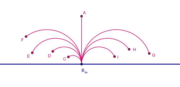
where s measures the length along a (possibly curved) line. The straight lines in the hyperbolic plane (geodesics for this metric tensor, i.e. curves which minimize the distance) are represented in this model by circular arcs perpendicular to the x-axis (half-circles whose origin is on the x-axis) and straight vertical rays perpendicular to the x-axis.

Distance calculation

In general, the distance between two points measured in this metric along such a geodesic is:

dist ⁡ ( ⟨ x 1 , y 1 ⟩ , ⟨ x 2 , y 2 ⟩ ) = arcosh ⁡ ( 1 + ( x 2 − x 1 ) 2 + ( y 2 − y 1 ) 2 2 y 1 y 2 ) .

Some special cases can be simplified:

dist ⁡ ( ⟨ x , y 1 ⟩ , ⟨ x , y 2 ⟩ ) = | ln ⁡ y 2 y 1 | = | ln ⁡ ( y 2 ) − ln ⁡ ( y 1 ) | . dist ⁡ ( ⟨ x 1 , y ⟩ , ⟨ x 2 , y ⟩ ) = | 2 arsinh ⁡ ( x 2 − x 1 2 y ) | dist ⁡ ( ⟨ x , r ⟩ , ⟨ x ± r sin ⁡ ϕ , r cos ⁡ ϕ ⟩ ) = arsinh ⁡ ( tan ⁡ ϕ ) = arcosh ⁡ ( 1 cos ⁡ ϕ ) = ln ⁡ ( 1 + sin ⁡ ϕ cos ⁡ ϕ )

where arcosh and arsinh are inverse hyperbolic functions

arsinh ⁡ x = ln ⁡ ( x + x 2 + 1 ) , arcosh ⁡ x = ln ⁡ ( x + x 2 − 1 ) ; x ≥ 1 .

Another way to calculate the distance between two points that are on an (Euclidean) half circle is:

dist ⁡ ( A B ) = | ln ⁡ ( | B A ∞ | | A B ∞ | | A A ∞ | | B B ∞ | ) | .

where A ∞ , B ∞ are the points where the halfcircles meet the boundary line and | P Q | is the euclidean length of the line segment connecting the points P and Q in the model.

Special points and curves

Ideal points (points at infinity) in the Poincaré half-plane model are of two kinds:

the points on the x-axis, and

one imaginary point at y = ∞ which is the ideal point to which all lines orthogonal to the x-axis converge.

Straight lines, geodesics (the shortest path between the points contained within it) are modeled by either:

half-circles whose origin is on the x-axis

straight vertical rays orthogonal to the x-axis

A circle (curves equidistant from a central point) with center ( x , y ) and radius r is modeled by:

An hypercycle (a curve equidistant from a straight line, its axis) is modeled by either:

a circular arc which intersects the x-axis at the same two ideal points as the half-circle which models its axis but at an acute or obtuse angle

a straight line which intersects the x-axis at the same point as the vertical line which models its axis , but at an acute or obtuse angle.

An horocycle (a curve whose normals all converge asymptotically in the same direction, its center) is modeled by either:

a circle tangent to the x-axis (but excluding the ideal point of intersection, which is its center)

a line parallel to the x-axis, in this case the center is the ideal point at y = ∞ .

Euclidean synopsis

A Euclidean circle with center ( x e , y e ) and radius r e represents:

when the circle is completely inside the halfplane a hyperbolic circle with center ( x e , y e 2 − r e 2 ) and radius 1 2 ln ⁡ ( y e + r e y e − r e )

when the circle is completely inside the halfplane and touches the boundary a horocycle centered around the ideal point ( x e , 0 )

when the circle intersects the boundary orthogonal ( y e = 0 ) a hyperbolic line

when the circle intersects the boundary non- orthogonal a hypercycle.

Compass and straightedge constructions

Here is how one can use compass and straightedge constructions in the model to achieve the effect of the basic constructions in the hyperbolic plane. For example, how to construct the half-circle in the Euclidean half-plane which models a line on the hyperbolic plane through two given points.

Creating the line through two existing points

Draw the line segment between the two points. Construct the perpendicular bisector of the line segment. Find its intersection with the x-axis. Draw the circle around the intersection which passes through the given points. Erase the part which is on or below the x-axis.

Or in the special case where the two given points lie on a vertical line, draw that vertical line through the two points and erase the part which is on or below the x-axis.

Creating the circle through one point with center another point

If the two points are not on a vertical line:

Draw the radial line (half-circle) between the two given points as in the previous case. Construct a tangent to that line at the non-central point. Drop a perpendicular from the given center point to the x-axis. Find the intersection of these two lines to get the center of the model circle. Draw the model circle around that new center and passing through the given non-central point.

If the two given points lie on a vertical line and the given center is above the other given point:

Draw a circle around the intersection of the vertical line and the x-axis which passes through the given central point. Draw a horizontal line through the non-central point. Construct the tangent to the circle at its intersection with that horizontal line.

The midpoint between the intersection of the tangent with the vertical line and the given non-central point is the center of the model circle. Draw the model circle around that new center and passing through the given non-central point.

If the two given points lie on a vertical line and the given center is below the other given point:

Draw a circle around the intersection of the vertical line and the x-axis which passes through the given central point. Draw a line tangent to the circle which passes through the given non-central point. Draw a horizontal line through that point of tangency and find its intersection with the vertical line.

The midpoint between that intersection and the given non-central point is the center of the model circle. Draw the model circle around that new center and passing through the given non-central point.

Given a circle find its (hyperbolic) center

Drop a perpendicular p from the Euclidean center of the circle to the x-axis.

Let point q be the intersection of this line and the x- axis.

Draw a line tangent to the circle going through q.

Draw the half circle h with center q going through the point where the tangent and the circle meet.

The (hyperbolic) center is the point where h and p intersect.

Other constructions

Creating the point which is the intersection of two existing lines, if they intersect:

Find the intersection of the two given semicircles (or vertical lines).

Creating the one or two points in the intersection of a line and a circle (if they intersect):

Find the intersection of the given semicircle (or vertical line) with the given circle.

Creating the one or two points in the intersection of two circles (if they intersect):

Find the intersection of the two given circles.

Symmetry groups

The projective linear group PGL(2,C) acts on the Riemann sphere by the Möbius transformations. The subgroup that maps the upper half-plane, H, onto itself is PSL(2,R), the transforms with real coefficients, and these act transitively and isometrically on the upper half-plane, making it a homogeneous space.

There are four closely related Lie groups that act on the upper half-plane by fractional linear transformations and preserve the hyperbolic distance.

The special linear group SL(2,R) which consists of the set of 2×2 matrices with real entries whose determinant equals +1. Note that many texts (including Wikipedia) often say SL(2,R) when they really mean PSL(2,R).

The group S*L(2,R) consisting of the set of 2×2 matrices with real entries whose determinant equals +1 or −1. Note that SL(2,R) is a subgroup of this group.

The projective special linear group PSL(2,R) = SL(2,R)/{±I}, consisting of the matrices in SL(2,R) modulo plus or minus the identity matrix.

The group PS^*L(2,R) = S^*L(2,R)/{±I}=PGL(2,R) is again a projective group, and again, modulo plus or minus the identity matrix. PSL(2,R) is contained as an index-two normal subgroup, the other coset being the set of 2×2 matrices with real entries whose determinant equals −1, modulo plus or minus the identity.

The relationship of these groups to the Poincaré model is as follows:

The group of all isometries of H, sometimes denoted as Isom(H), is isomorphic to PS^*L(2,R). This includes both the orientation preserving and the orientation-reversing isometries. The orientation-reversing map (the mirror map) is z → − z ¯ .

The group of orientation-preserving isometries of H, sometimes denoted as Isom⁺(H), is isomorphic to PSL(2,R).

Important subgroups of the isometry group are the Fuchsian groups.

One also frequently sees the modular group SL(2,Z). This group is important in two ways. First, it is a symmetry group of the square 2x2 lattice of points. Thus, functions that are periodic on a square grid, such as modular forms and elliptic functions, will thus inherit an SL(2,Z) symmetry from the grid. Second, SL(2,Z) is of course a subgroup of SL(2,R), and thus has a hyperbolic behavior embedded in it. In particular, SL(2,Z) can be used to tessellate the hyperbolic plane into cells of equal (Poincaré) area.

Isometric symmetry

The group action of the projective special linear group PSL(2,R) on H is defined by

( a b c d ) ⋅ z = a z + b c z + d = ( a c | z | 2 + b d + ( a d + b c ) ℜ ( z ) ) + i ( a d − b c ) ℑ ( z ) | c z + d | 2 .

Note that the action is transitive, in that for any z 1 , z 2 ∈ H , there exists a g ∈ P S L ( 2 , R ) such that g z 1 = z 2 . It is also faithful, in that if g z = z for all z in H, then g=e.

The stabilizer or isotropy subgroup of an element z in H is the set of g ∈ P S L ( 2 , R ) which leave z unchanged: gz=z. The stabilizer of i is the rotation group

S O ( 2 ) = { ( cos ⁡ θ sin ⁡ θ − sin ⁡ θ cos ⁡ θ ) : θ ∈ R } .

Since any element z in H is mapped to i by some element of PSL(2,R), this means that the isotropy subgroup of any z is isomorphic to SO(2). Thus, H = PSL(2,R)/SO(2). Alternatively, the bundle of unit-length tangent vectors on the upper half-plane, called the unit tangent bundle, is isomorphic to PSL(2,R).

The upper half-plane is tessellated into free regular sets by the modular group SL(2,Z).

Geodesics

The geodesics for this metric tensor are circular arcs perpendicular to the real axis (half-circles whose origin is on the real axis) and straight vertical lines ending on the real axis.

The unit-speed geodesic going up vertically, through the point i is given by

γ ( t ) = ( e t / 2 0 0 e − t / 2 ) ⋅ i = i e t .

Because PSL(2,R) acts transitively by isometries of the upper half-plane, this geodesic is mapped into the other geodesics through the action of PSL(2,R). Thus, the general unit-speed geodesic is given by

γ ( t ) = ( a b c d ) ( e t / 2 0 0 e − t / 2 ) ⋅ i = a i e t + b c i e t + d .

This provides the complete description of the geodesic flow on the unit-length tangent bundle (complex line bundle) on the upper half-plane.

The model in three dimensions

The metric of the model on the half- space

{ ⟨ x , y , z ⟩ | z > 0 }

is given by

( d s ) 2 = ( d x ) 2 + ( d y ) 2 + ( d z ) 2 z 2

where s measures length along a possibly curved line. The straight lines in the hyperbolic space (geodesics for this metric tensor, i.e. curves which minimize the distance) are represented in this model by circular arcs normal to the z = 0-plane (half-circles whose origin is on the z = 0-plane) and straight vertical rays normal to the z = 0-plane.

The distance between two points measured in this metric along such a geodesic is:

dist ⁡ ( ⟨ x 1 , y 1 , z 1 ⟩ , ⟨ x 2 , y 2 , z 2 ⟩ ) = arcosh ⁡ ( 1 + ( x 2 − x 1 ) 2 + ( y 2 − y 1 ) 2 + ( z 2 − z 1 ) 2 2 z 1 z 2 ) .

The model in n dimensions

This model can be generalized to model an n+1 dimensional hyperbolic space by replacing the real number x by a vector in an n dimensional Euclidean vector space.

References

Poincaré half-plane model Wikipedia

(Text) CC BY-SA

Contents