Pearson correlation coefficient

Definition

Pearson's correlation coefficient is the covariance of the two variables divided by the product of their standard deviations. The form of the definition involves a "product moment", that is, the mean (the first moment about the origin) of the product of the mean-adjusted random variables; hence the modifier product-moment in the name.

For a population

Pearson's correlation coefficient when applied to a population is commonly represented by the Greek letter ρ (rho) and may be referred to as the population correlation coefficient or the population Pearson correlation coefficient. The formula for ρ is:

ρ X , Y = cov ⁡ ( X , Y ) σ X σ Y

The formula for ρ can be expressed in terms of mean and expectation. Since

cov ⁡ ( X , Y ) = E ⁡ [ ( X − μ X ) ( Y − μ Y ) ]

Then the formula for ρ can also be written as

ρ X , Y = E ⁡ [ ( X − μ X ) ( Y − μ Y ) ] σ X σ Y

The formula for ρ can be expressed in terms of uncentered moments. Since

the formula for ρ can also be written as

ρ X , Y = E ⁡ [ X Y ] − E ⁡ [ X ] E ⁡ [ Y ] E ⁡ [ X 2 ] − [ ⁡ E [ X ] ] 2   E ⁡ [ Y 2 ] − [ ⁡ E [ Y ] ] 2 .

For a sample

Pearson's correlation coefficient when applied to a sample is commonly represented by the letter r and may be referred to as the sample correlation coefficient or the sample Pearson correlation coefficient. We can obtain a formula for r by substituting estimates of the covariances and variances based on a sample into the formula above. So if we have one dataset {x₁,...,x_n} containing n values and another dataset {y₁,...,y_n} containing n values then that formula for r is:

r = ∑ i = 1 n ( x i − x ¯ ) ( y i − y ¯ ) ∑ i = 1 n ( x i − x ¯ ) 2 ∑ i = 1 n ( y i − y ¯ ) 2

Rearranging gives us this formula for r:

r = r x y = n ∑ x i y i − ∑ x i ∑ y i n ∑ x i 2 − ( ∑ x i ) 2   n ∑ y i 2 − ( ∑ y i ) 2 .

Rearranging again gives us this formula for r:

r = r x y = ∑ x i y i − n x ¯ y ¯ ( ∑ x i 2 − n x ¯ 2 )   ( ∑ y i 2 − n y ¯ 2 ) .

An equivalent expression gives the formula for r as the mean of the products of the standard scores as follows:

r = r x y = 1 n − 1 ∑ i = 1 n ( x i − x ¯ s x ) ( y i − y ¯ s y )

Alternative formulae for r are also available. One can use the following formula for r:

r = r x y = ∑ x i y i − n x ¯ y ¯ ( n − 1 ) s x s y

Practical issues

Under heavy noise conditions, extracting the correlation coefficient between two sets of stochastic variables is nontrivial, in particular where Canonical Correlation Analysis reports on degraded correlation values due to the heavy noise contributions. A generalization of the approach is given elsewhere.

In case of missing data, Garren derived the maximum likelihood estimator.

Mathematical properties

The absolute values of both the sample and population Pearson correlation coefficients are less than or equal to 1. Correlations equal to 1 or −1 correspond to data points lying exactly on a line (in the case of the sample correlation), or to a bivariate distribution entirely supported on a line (in the case of the population correlation). The Pearson correlation coefficient is symmetric: corr(X,Y) = corr(Y,X).

A key mathematical property of the Pearson correlation coefficient is that it is invariant to separate changes in location and scale in the two variables. That is, we may transform X to a + bX and transform Y to c + dY, where a, b, c, and d are constants with b, d ≠ 0, without changing the correlation coefficient. (This fact holds for both the population and sample Pearson correlation coefficients.) Note that more general linear transformations do change the correlation: see a later section for an application of this.

Interpretation

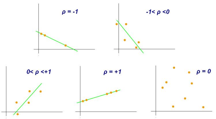
The correlation coefficient ranges from −1 to 1. A value of 1 implies that a linear equation describes the relationship between X and Y perfectly, with all data points lying on a line for which Y increases as X increases. A value of −1 implies that all data points lie on a line for which Y decreases as X increases. A value of 0 implies that there is no linear correlation between the variables.

More generally, note that (X_i − X)(Y_i − Y) is positive if and only if X_i and Y_i lie on the same side of their respective means. Thus the correlation coefficient is positive if X_i and Y_i tend to be simultaneously greater than, or simultaneously less than, their respective means. The correlation coefficient is negative (anti-correlation) if X_i and Y_i tend to lie on opposite sides of their respective means. Moreover, the stronger is either tendency, the larger is the absolute value of the correlation coefficient.

Geometric interpretation

For uncentered data, there is a relation between the correlation coefficient and the angle φ between the two regression lines, y=g_x(x) and x=g_y(y), obtained by regressing y on x and x on y respectively. (Here φ is measured within the first quadrant formed around the lines' intersection point if r > 0, or counterclockwise from the fourth to the second quadrant if r < 0.) One can show that if the standard deviations are equal, then r = sec   φ – tan   φ , where sec and tan are trigonometric functions.

For centered data (i.e., data which have been shifted by the sample means of their respective variables so as to have an average of zero for each variable), the correlation coefficient can also be viewed as the cosine of the angle   θ between the two vectors of samples in N-dimensional space (for N samples of each variable) (as illustrated for a special case in the next paragraph).

Both the uncentered (non-Pearson-compliant) and centered correlation coefficients can be determined for a dataset. As an example, suppose five countries are found to have gross national products of 1, 2, 3, 5, and 8 billion dollars, respectively. Suppose these same five countries (in the same order) are found to have 11%, 12%, 13%, 15%, and 18% poverty. Then let x and y be ordered 5-element vectors containing the above data: x = (1, 2, 3, 5, 8) and y = (0.11, 0.12, 0.13, 0.15, 0.18).

By the usual procedure for finding the angle   θ between two vectors (see dot product), the uncentered correlation coefficient is:

cos ⁡ θ = x ⋅ y ∥ x ∥ ∥ y ∥ = 2.93 103 0.0983 = 0.920814711.

This uncentred correlation coefficient is identical with the cosine similarity. Note that the above data were deliberately chosen to be perfectly correlated: y = 0.10 + 0.01 x. The Pearson correlation coefficient must therefore be exactly one. Centering the data (shifting x by E(x) = 3.8 and y by E(y) = 0.138) yields x = (−2.8, −1.8, −0.8, 1.2, 4.2) and y = (−0.028, −0.018, −0.008, 0.012, 0.042), from which

cos ⁡ θ = x ⋅ y ∥ x ∥ ∥ y ∥ = 0.308 30.8 0.00308 = 1 = ρ x y ,

as expected.

Interpretation of the size of a correlation

Several authors have offered guidelines for the interpretation of a correlation coefficient. However, all such criteria are in some ways arbitrary and should not be observed too strictly. The interpretation of a correlation coefficient depends on the context and purposes. A correlation of 0.8 may be very low if one is verifying a physical law using high-quality instruments, but may be regarded as very high in the social sciences where there may be a greater contribution from complicating factors.

Inference

Statistical inference based on Pearson's correlation coefficient often focuses on one of the following two aims:

One aim is to test the null hypothesis that the true correlation coefficient ρ is equal to 0, based on the value of the sample correlation coefficient r.

The other aim is to derive a confidence interval that, on repeated sampling, has a given probability of containing ρ.

We discuss methods of achieving one or both of these aims below.

Using a permutation test

Permutation tests provide a direct approach to performing hypothesis tests and constructing confidence intervals. A permutation test for Pearson's correlation coefficient involves the following two steps:

1. Using the original paired data (x_i, y_i), randomly redefine the pairs to create a new data set (x_i, y_i′), where the i′ are a permutation of the set {1,...,n}. The permutation i′ is selected randomly, with equal probabilities placed on all n! possible permutations. This is equivalent to drawing the i′ randomly "without replacement" from the set {1, ..., n}. A closely related and equally justified (bootstrapping) approach is to separately draw the i and the i′ "with replacement" from {1, ..., n};
2. Construct a correlation coefficient r from the randomized data.

To perform the permutation test, repeat steps (1) and (2) a large number of times. The p-value for the permutation test is the proportion of the r values generated in step (2) that are larger than the Pearson correlation coefficient that was calculated from the original data. Here "larger" can mean either that the value is larger in magnitude, or larger in signed value, depending on whether a two-sided or one-sided test is desired.

Using a bootstrap

The bootstrap can be used to construct confidence intervals for Pearson's correlation coefficient. In the "non-parametric" bootstrap, n pairs (x_i, y_i) are resampled "with replacement" from the observed set of n pairs, and the correlation coefficient r is calculated based on the resampled data. This process is repeated a large number of times, and the empirical distribution of the resampled r values are used to approximate the sampling distribution of the statistic. A 95% confidence interval for ρ can be defined as the interval spanning from the 2.5^th to the 97.5^th percentile of the resampled r values.

Testing using Student's t-distribution

For pairs from an uncorrelated bivariate normal distribution, the sampling distribution of a certain function of Pearson's correlation coefficient follows Student's t-distribution with degrees of freedom n − 2. Specifically, if the underlying variables have a bivariate normal distribution, the variable

t = r n − 2 1 − r 2

has a Student's t-distribution in the null case (zero correlation). This also holds approximately even if the observed values are non-normal, provided sample sizes are not very small. For determining the critical values for r the inverse of this transformation is also needed:

r = t n − 2 + t 2 .

Alternatively, large sample approaches can be used.

Early work on the distribution of the sample correlation coefficient was carried out by Anil Kumar Gain and R. A. Fisher

Another early paper provides graphs and tables for general values of ρ, for small sample sizes, and discusses computational approaches.

Using the exact distribution

For data that follows a bivariate normal distribution, the exact density function f(r) for the sample correlation coefficient r of a normal bivariate is

f ( r ) = ( n − 2 ) Γ ( n − 1 ) ( 1 − ρ 2 ) n − 1 2 ( 1 − r 2 ) n − 4 2 2 π Γ ( n − 1 2 ) ( 1 − ρ r ) n − 3 2 2 F 1 ( 1 2 , 1 2 ; 2 n − 1 2 ; ρ r + 1 2 )

In the special case when ρ = 0 , the exact density function f(r) can be written as:

f ( r ) = ( 1 − r 2 ) n − 4 2 B ( 1 2 , n − 2 2 ) ,

Using the Fisher transformation

In practice, confidence intervals and hypothesis tests relating to ρ are usually carried out using the Fisher transformation:

F ( r ) = 1 2 ln ⁡ 1 + r 1 − r = arctanh ⁡ ( r ) .

If F(r) is the Fisher transformation of r, and n is the sample size, then F(r) approximately follows a normal distribution with

mean = F ( ρ ) = artanh ⁡ ( ρ )     and standard error     SE = 1 n − 3 .

Thus, a z-score is

z = x − mean SE = [ F ( r ) − F ( ρ 0 ) ] n − 3

under the null hypothesis of that ρ = ρ 0 , given the assumption that the sample pairs are independent and identically distributed and follow a bivariate normal distribution. Thus an approximate p-value can be obtained from a normal probability table. For example, if z = 2.2 is observed and a two-sided p-value is desired to test the null hypothesis that ρ = 0 , the p-value is 2·Φ(−2.2) = 0.028, where Φ is the standard normal cumulative distribution function.

To obtain a confidence interval for ρ, we first compute a confidence interval for F( ρ ):

100 ( 1 − α ) % CI : artanh ⁡ ( ρ ) ∈ [ artanh ⁡ ( r ) ± z α / 2 S E ]

The inverse Fisher transformation bring the interval back to the correlation scale.

100 ( 1 − α ) % CI : ρ ∈ [ tanh ⁡ ( artanh ⁡ ( r ) − z α / 2 S E ) , tanh ⁡ ( artanh ⁡ ( r ) + z α / 2 S E ) ]

For example, suppose we observe r = 0.3 with a sample size of n=50, and we wish to obtain a 95% confidence interval for ρ. The transformed value is artanh(r) = 0.30952, so the confidence interval on the transformed scale is 0.30952 ± 1.96/√47, or (0.023624, 0.595415). Converting back to the correlation scale yields (0.024, 0.534).

In least squares regression analysis

The square of the sample correlation coefficient is typically denoted r² and is a special case of the coefficient of determination. In this case, it estimates the fraction of the variance in Y that is explained by X in a simple linear regression. So if we have the observed dataset {y₁,...,y_n} and the fitted dataset {f₁,...,f_n}, and we denote the fitted dataset {f₁,...,f_n} with {ŷ₁,...,ŷ_n}, then as a starting point the total variation in the Y_i around their average value can be decomposed as follows

∑ i ( Y i − Y ¯ ) 2 = ∑ i ( Y i − Y ^ i ) 2 + ∑ i ( Y ^ i − Y ¯ ) 2 ,

where the Y ^ i are the fitted values from the regression analysis. This can be rearranged to give

1 = ∑ i ( Y i − Y ^ i ) 2 ∑ i ( Y i − Y ¯ ) 2 + ∑ i ( Y ^ i − Y ¯ ) 2 ∑ i ( Y i − Y ¯ ) 2 .

The two summands above are the fraction of variance in Y that is explained by X (right) and that is unexplained by X (left).

Next, we apply a property of least square regression models, that the sample covariance between Y ^ i and Y i − Y ^ i is zero. Thus, the sample correlation coefficient between the observed and fitted response values in the regression can be written (calculation is under expectation, assumes Gaussian statistics)

r ( Y , Y ^ ) = ∑ i ( Y i − Y ¯ ) ( Y ^ i − Y ¯ ) ∑ i ( Y i − Y ¯ ) 2 ⋅ ∑ i ( Y ^ i − Y ¯ ) 2 = ∑ i ( Y i − Y ^ i + Y ^ i − Y ¯ ) ( Y ^ i − Y ¯ ) ∑ i ( Y i − Y ¯ ) 2 ⋅ ∑ i ( Y ^ i − Y ¯ ) 2 = ∑ i [ ( Y i − Y ^ i ) ( Y ^ i − Y ¯ ) + ( Y ^ i − Y ¯ ) 2 ] ∑ i ( Y i − Y ¯ ) 2 ⋅ ∑ i ( Y ^ i − Y ¯ ) 2 = ∑ i ( Y ^ i − Y ¯ ) 2 ∑ i ( Y i − Y ¯ ) 2 ⋅ ∑ i ( Y ^ i − Y ¯ ) 2 = ∑ i ( Y ^ i − Y ¯ ) 2 ∑ i ( Y i − Y ¯ ) 2 .

Thus

r ( Y , Y ^ ) 2 = ∑ i ( Y ^ i − Y ¯ ) 2 ∑ i ( Y i − Y ¯ ) 2

That equation can be written as:

r ( Y , Y ^ ) 2 = S S reg S S tot

Existence

The population Pearson correlation coefficient is defined in terms of moments, and therefore exists for any bivariate probability distribution for which the population covariance is defined and the marginal population variances are defined and are non-zero. Some probability distributions such as the Cauchy distribution have undefined variance and hence ρ is not defined if X or Y follows such a distribution. In some practical applications, such as those involving data suspected to follow a heavy-tailed distribution, this is an important consideration. However, the existence of the correlation coefficient is usually not a concern; for instance, if the range of the distribution is bounded, ρ is always defined.

Sample size

If the sample size is moderate or large and the population is normal then in the case of the bivariate normal distribution, the sample correlation coefficient is the maximum likelihood estimate of the population correlation coefficient, and is asymptotically unbiased and efficient, which roughly means that it is impossible to construct a more accurate estimate than the sample correlation coefficient.

If the sample size is large and the population is not normal, then the sample correlation coefficient remains approximately unbiased, but may not be efficient.

If the sample size is large then sample correlation coefficient is a consistent estimator of the population correlation coefficient as long as the sample means, variances, and covariance are consistent (which is guaranteed when the law of large numbers can be applied).

If the sample size is small then the sample correlation coefficient r is not an unbiased estimate of ρ. The adjusted correlation coefficient must be used instead: see elsewhere in this article for the definition.

Robustness

Like many commonly used statistics, the sample statistic r is not robust, so its value can be misleading if outliers are present. Specifically, the PMCC is neither distributionally robust, nor outlier resistant (see Robust statistics#Definition). Inspection of the scatterplot between X and Y will typically reveal a situation where lack of robustness might be an issue, and in such cases it may be advisable to use a robust measure of association. Note however that while most robust estimators of association measure statistical dependence in some way, they are generally not interpretable on the same scale as the Pearson correlation coefficient.

Statistical inference for Pearson's correlation coefficient is sensitive to the data distribution. Exact tests, and asymptotic tests based on the Fisher transformation can be applied if the data are approximately normally distributed, but may be misleading otherwise. In some situations, the bootstrap can be applied to construct confidence intervals, and permutation tests can be applied to carry out hypothesis tests. These non-parametric approaches may give more meaningful results in some situations where bivariate normality does not hold. However the standard versions of these approaches rely on exchangeability of the data, meaning that there is no ordering or grouping of the data pairs being analyzed that might affect the behavior of the correlation estimate.

A stratified analysis is one way to either accommodate a lack of bivariate normality, or to isolate the correlation resulting from one factor while controlling for another. If W represents cluster membership or another factor that it is desirable to control, we can stratify the data based on the value of W, then calculate a correlation coefficient within each stratum. The stratum-level estimates can then be combined to estimate the overall correlation while controlling for W.

Variants

Variations of the correlation coefficient can be calculated for different purposes. Here are some examples.

Adjusted correlation coefficient

The sample correlation coefficient r is not an unbiased estimate of ρ. For data that follows a bivariate normal distribution, the expectation E(r) for the sample correlation coefficient r of a normal bivariate is

E ⁡ [ r ] = ρ − ρ ( 1 − ρ 2 ) 2 n + ⋯ , therefore r is a biased estimator of ρ .

The unique minimum variance unbiased estimator r_adj is given by

( 1 ) r adj = r 2 F 1 ( 1 2 , 1 2 ; n − 1 2 ; 1 − r 2 ) ,

An approximately unbiased estimator r_adj can be obtained by truncating E[r] and solving this truncated equation:

( 2 ) r = E ⁡ [ r ] = r adj − r adj ( 1 − r adj 2 ) 2 n .

The solution to equation (2) is:

( 3 ) r a d j = r [ 1 + 1 − r 2 2 n ] ,

Another proposed adjusted correlation coefficient is:

r adj = 1 − ( 1 − r 2 ) ( n − 1 ) ( n − 2 ) .

Note that r_adj ≈ r for large values of n.

Weighted correlation coefficient

Suppose observations to be correlated have differing degrees of importance that can be expressed with a weight vector w. To calculate the correlation between vectors x and y with the weight vector w (all of length n),

Weighted mean:

Weighted covariance

Weighted correlation

Reflective correlation coefficient

The reflective correlation is a variant of Pearson's correlation in which the data are not centered around their mean values. The population reflective correlation is

Corr r ( X , Y ) = E [ X Y ] E X 2 ⋅ E Y 2 .

The reflective correlation is symmetric, but it is not invariant under translation:

Corr r ( X , Y ) = Corr r ( Y , X ) = Corr r ( X , b Y ) ≠ Corr r ( X , a + b Y ) , a ≠ 0 , b > 0.

The sample reflective correlation is

r r x y = ∑ x i y i ( ∑ x i 2 ) ( ∑ y i 2 ) .

The weighted version of the sample reflective correlation is

r r x y , w = ∑ w i x i y i ( ∑ w i x i 2 ) ( ∑ w i y i 2 ) .

Scaled correlation coefficient

Scaled correlation is a variant of Pearson's correlation in which the range of the data is restricted intentionally and in a controlled manner to reveal correlations between fast components in time series. Scaled correlation is defined as average correlation across short segments of data.

Let K be the number of segments that can fit into the total length of the signal T for a given scale s :

K = round ⁡ ( T s ) .

The scaled correlation across the entire signals r ¯ s is then computed as

r ¯ s = 1 K ∑ k = 1 K r k ,

where r k is Pearson's coefficient of correlation for segment k .

By choosing the parameter s , the range of values is reduced and the correlations on long time scale are filtered out, only the correlations on short time scales being revealed. Thus, the contributions of slow components are removed and those of fast components are retained.

Pearson's distance

A distance metric for two variables X and Y known as Pearson's distance can be defined from their correlation coefficient as

d X , Y = 1 − ρ X , Y .

Considering that the Pearson correlation coefficient falls between [−1, 1], the Pearson distance lies in [0, 2].

Circular correlation coefficient

For variables X = {x₁,...,x_n} and Y = {y₁,...,y_n} that are defined on the unit circle [0, 2π), it is possible to define a circular analog of Pearson's coefficient. This is done by transforming data points in X and Y with a sine function such that the correlation coefficient is given as:

r circular = ∑ i = 1 n sin ⁡ ( x i − x ¯ ) sin ⁡ ( y i − y ¯ ) ∑ i = 1 n sin ⁡ ( x i − x ¯ ) 2 ∑ i = 1 n sin ⁡ ( y i − y ¯ ) 2

where x ¯ and y ¯ are the circular means of X and Y. This measure can be useful in fields like meteorology where the angular direction of data is important.

Partial correlation

If a population or data-set is characterized by more than two variables, a partial correlation coefficient measures the strength of dependence between a pair of variables that is not accounted for by the way in which they both change in response to variations in a selected subset of the other variables.

Decorrelation

It is always possible to remove the correlation between random variables with a linear transformation, even if the relationship between the variables is nonlinear. A presentation of this result for population distributions is given by Cox & Hinkley.

A corresponding result exists for sample correlations, in which the sample correlation is reduced to zero. Suppose a vector of n random variables is sampled m times. Let X be a matrix where X i , j is the jth variable of sample i. Let Z m , m be an m by m square matrix with every element 1. Then D is the data transformed so every random variable has zero mean, and T is the data transformed so all variables have zero mean and zero correlation with all other variables – the sample covariance matrix of T will be the identity matrix. This has to be further divided by the standard deviation to get unit variance. The transformed variables will be uncorrelated, even though they may not be independent.

D = X − 1 m Z m , m X T = D ( D T D ) − 1 2 ,

where an exponent of −1/2 represents the matrix square root of the inverse of a matrix. The covariance matrix of T will be the identity matrix. If a new data sample x is a row vector of n elements, then the same transform can be applied to x to get the transformed vectors d and t:

d = x − 1 m Z 1 , m X , t = d ( D T D ) − 1 2 .

This decorrelation is related to principal components analysis for multivariate data.