Parks–McClellan filter design algorithm

History of optimal FIR filter design

In the 1960s, researchers within the field of analog filter design were using the Chebyshev approximation for filter design. During this time, it was well known that the best filters contain an equiripple characteristic in their frequency response magnitude and the elliptic filter (or Cauer filter) was optimal with regards to the Chebyshev approximation. When the digital filter revolution began in the 1960s, researchers used a bilinear transform to produce infinite impulse response (IIR) digital elliptic filters. They also recognized the potential for designing FIR filters to accomplish the same filtering task and soon the search was on for the optimal FIR filter using the Chebyshev approximation.

It was well known in both mathematics and engineering that the optimal response would exhibit an equiripple behavior and that the number of ripples could be counted using the Chebyshev approximation. Several attempts to produce a design program for the optimal Chebyshev FIR filter were undertaken in the period between 1962 and 1971. Despite the numerous attempts, most did not succeed, usually due to problems in the algorithmic implementation or problem formulation. Otto Herrmann, for example, proposed a method for designing equiripple filters with restricted band edges. This method obtained an equiripple frequency response with the maximum number of ripples by solving a set of nonlinear equations. Another method introduced at the time implemented an optimal Chebyshev approximation, but the algorithm was limited to the design of relatively low-order filters.

Similar to Herrmann's method, Ed Hofstetter presented an algorithm that designed FIR filters with as many ripples as possible. This has become known as the Maximal Ripple algorithm. The Maximal Ripple algorithm imposed an alternating error condition via interpolation and then solved a set of equations that the alternating solution had to satisfy. One notable limitation of the Maximal Ripple algorithm was that the band edges were not specified as inputs to the design procedure. Rather, the initial frequency set {ω_i} and the desired function D(ω_i) defined the pass and stop band implicitly. Unlike previous attempts to design an optimal filter, the Maximal Ripple algorithm used an exchange method that tried to find the frequency set {ω_i} where the best filter had its ripples. Thus, the Maximal Ripple algorithm was not an optimal filter design but it had quite a significant impact on how the Parks–McClellan algorithm would formulate.

History

In August 1970, James McClellan entered graduate school at Rice University with a concentration in mathematical models of analog filter design. James McClellan enrolled in a new course called "Digital Filters" due to his interest in filter design. The course was taught jointly by Thomas Parks and Sid Burrus. At that time, DSP was an emerging field and, as a result, lectures often involved recently published research papers. The following semester, the spring of 1971, Thomas Parks offered a course called "Signal Theory," which James McClellan took as well. During spring break of the semester, Thomas drove from Houston to Princeton in order to attend a conference. At the conference, he heard Ed Hofstetter's presentation about a new FIR filter design algorithm (Maximal Ripple algorithm). He brought the paper by Hofstetter, Oppenheim, and Siegel, back to Houston, thinking about the possibility of using the Chebyshev approximation theory to design FIR filters. He heard that the method implemented in Hofstetter's algorithm was similar to the Remez exchange algorithm and decided to pursue the path of using the Remez exchange algorithm. The students in the "Signal Theory" course were required to do a project and since Chebyshev approximation was a major topic in the course, the implementation of this new algorithm became James McClellan's course project. This ultimately led to the Parks–McClellan algorithm, which involved the theory of optimal Chebyshev approximation and an efficient implementation. By the end of the spring semester, James McClellan and Thomas Parks were attempting to write a variation of the Remez exchange algorithm for FIR filters. It took about six weeks to develop and by the end of May, some optimal filters had been designed successfully.

James McClellan and Thomas Parks

James McClellan was born on October 5, 1947 in Guam. He received his Bachelor of Science in Electrical Engineering (1969) from Louisiana State University. After receiving his Master of Science (1972) and Doctorate (1973) degrees from Rice University, Dr. McClellan worked at the MIT Lincoln Laboratory from 1973 to 1975. He became a professor in the MIT Electrical Engineering and Computer Science Department in 1975. After working at the university for seven years, Dr. McClellan joined Schlumberger in 1982, where he worked for five years. Since 1987, Dr. McClellan has been a Professor of Electrical Engineering at the Georgia Institute of Technology. Dr. McClellan has received numerous awards for his work in digital signal processing and its application to sensor array processing: IEEE Signal Processing Technical Achievement Award (1987), IEEE Signal Processing Society Award (1996), and IEEE Jack S. Kilby Signal Processing Medal (2004). In addition to the awards he has received, Dr. McClellan has published a number of significant pieces of literature: Computer-Based Exercises for Signal Processing Using MATLAB 5 (1994), DSP First (1997), Signal Processing First (2003), and Number Theory in DSP (1979).

Thomas Parks was born on March 16, 1939 in Buffalo, New York. He received his Bachelor (1961), Master of Science (1964), and Doctorate (1967) degrees in Electrical Engineering from Cornell University. After graduating with his doctorate, Dr. Parks joined the faculty at Rice University. He was a faculty member from 1967 to 1986, when he joined the faculty at Cornell University. Dr. Parks is the recipient of multiple awards based on his research focused on digital signal processing with its application to signal theory, multirate systems, interpolation, and filter design: IEEE ASSP Society Technical Achievement Award (1981), IEEE ASSP Society Award (1988), Rice University President's Award (1999), IEEE Third Millennium Medal (2000), and IEEE Jack S. Kilby Signal Processing Medal (2004). In addition to the awards he has received, Dr. Parks has published numerous contributions to the electrical engineering field: DFT/FFT Convolution Algorithms (1985), Digital Filter Design (1987), A Digital Signal Processing Laboratory Using the TMS 32010 (1988), A Digital Signal Processing Laboratory Using the TMS 320C25 (1990), Computer-Based Exercises for Signal Processing (1994), and Computer-Based Exercises for Signal Processing Using MATLAB 5 (1994).

The algorithm

The Parks–McClellan Algorithm is implemented using the following steps:

1. Initialization: Choose an extremal set of frequences {ω_i⁽⁰⁾}.
2. Finite Set Approximation: Calculate the best Chebyshev approximation on the present extremal set, giving a value δ^(m) for the min-max error on the present extremal set.
3. Interpolation: Calculate the error function E(ω) over the entire set of frequencies Ω using (2).
4. Look for local maxima of |E^(m)(ω)| on the set Ω.
5. If max_(ωεΩ)|E^(m)(ω)| > δ^(m), then update the extremal set to {ω_i^(m+1)} by picking new frequencies where |E^(m)(ω)| has its local maxima. Make sure that the error alternates on the ordered set of frequencies as described in (4) and (5). Return to Step 2 and iterate.
6. If max_(ωεΩ)|E^(m)(ω)| ≤ δ^(m), then the algorithm is complete. Use the set {ω_i⁽⁰⁾} and the interpolation formula to compute an inverse discrete Fourier transform to obtain the filter coefficients.

The Parks–McClellan Algorithm may be restated as the following steps:

1. Make an initial guess of the L+2 extremal frequencies.
2. Compute δ using the equation given.
3. Using Lagrange Interpolation, we compute the dense set of samples of A(ω) over the passband and stopband.
4. Determine the new L+2 largest extrema.
5. If the alternation theorem is not satisfied, then we go back to (2) and iterate until the alternation theorem is satisfied.
6. If the alternation theorem is satisfied, then we compute h(n) and we are done.

To gain a basic understanding of the Parks–McClellan Algorithm mentioned above, we can rewrite the algorithm above in a simpler form as:

1. Guess the positions of the extrema are evenly spaced in the pass and stop band.
2. Perform polynomial interpolation and re-estimate positions of the local extrema.
3. Move extrema to new positions and iterate until the extrema stop shifting.

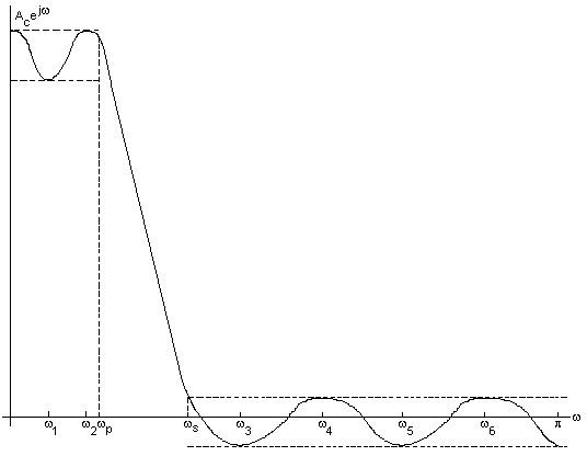
Explanation

The picture above on the right displays the various extremal frequencies for the plot shown. The extremal frequencies are the maximum and minimum points in the stop and pass bands. The stop band ripple is the lower portion of ripples on the bottom right of the plot and the pass band ripple is the upper portion of the ripples on the top left of the plot. The dashed lines going across the plot indicate the δ or maximum error. Given the positions of the extremal frequencies, there is a formula for the optimum δ or optimum error. Since we do not know the optimum δ or the exact positions of the extrema on the first attempt, we iterate. Effectively, we assume the positions of the extrema initially, and calculate δ. We then re-estimate and move the extrema and recalculate δ, or the error. We repeat this process until δ stops changing. The algorithm will cause the δ error to converge, generally within ten to twelve iterations.