Otsu's method - Alchetron, The Free Social Encyclopedia

In computer vision and image processing, Otsu's method, named after Nobuyuki Otsu (大津展之, Ōtsu Nobuyuki), is used to automatically perform clustering-based image thresholding, or, the reduction of a graylevel image to a binary image. The algorithm assumes that the image contains two classes of pixels following bi-modal histogram (foreground pixels and background pixels), it then calculates the optimum threshold separating the two classes so that their combined spread (intra-class variance) is minimal, or equivalently (because the sum of pairwise squared distances is constant), so that their inter-class variance is maximal. Consequently, Otsu's method is roughly a one-dimensional, discrete analog of Fisher's Discriminant Analysis. Otsu's method is also directly related to the Jenks optimization method.

Method

In Otsu's method we exhaustively search for the threshold that minimizes the intra-class variance (the variance within the class), defined as a weighted sum of variances of the two classes:

σ w 2 ( t ) = ω 0 ( t ) σ 0 2 ( t ) + ω 1 ( t ) σ 1 2 ( t )

Weights ω 0 and ω 1 are the probabilities of the two classes separated by a threshold t and σ 0 2 and σ 1 2 are variances of these two classes.

The class probability ω 0 , 1 ( t ) is computed from the L histograms:

ω 0 ( t ) = ∑ i = 0 t − 1 p ( i ) ω 1 ( t ) = ∑ i = t L − 1 p ( i )

Otsu shows that minimizing the intra-class variance is the same as maximizing inter-class variance:

σ b 2 ( t ) = σ 2 − σ w 2 ( t ) = ω 0 ( μ 0 − μ T ) 2 + ω 1 ( μ 1 − μ T ) 2 = ω 0 ( t ) ω 1 ( t ) [ μ 0 ( t ) − μ 1 ( t ) ] 2

which is expressed in terms of class probabilities ω and class means μ .

while the class mean μ 0 , 1 , T ( t ) is:

μ 0 ( t ) = ∑ i = 0 t − 1 i p ( i ) ω 0 μ 1 ( t ) = ∑ i = t L − 1 i p ( i ) ω 1 μ T = ∑ i = 0 L − 1 i p ( i )

The following relations can be easily verified:

ω 0 μ 0 + ω 1 μ 1 = μ T ω 0 + ω 1 = 1

The class probabilities and class means can be computed iteratively. This idea yields an effective algorithm.

Algorithm

Compute histogram and probabilities of each intensity level
Set up initial ω i ( 0 ) and μ i ( 0 )
Step through all possible thresholds t = 1 , … maximum intensity
1. Update ω i and μ i
2. Compute σ b 2 ( t )
Desired threshold corresponds to the maximum σ b 2 ( t )

MATLAB implementation

histogramCounts is a 256-element histogram of a grayscale image different gray-levels (typical for 8-bit images). level is the threshold for the image (double).

Matlab have built-in functions graythresh() and multithresh() in Image Processing Toolbox which are implemented with Otsu's method and Multi Otsu's method, respectively.

Another approach with vectorized method (could be easily converted into python matrix-array version for GPU processing)

The implementation has a little redundancy of computation. But since Otsu method is fast, the implementation is acceptable and easy to understand. While in some environment, since we employ vectorisation form, loop computation might be faster. This method can be easily converted to multi-threshold method, with architecture minimum heap—children labels.

Variant 1

NB: The input argument total is the number of pixels in the given image. The input argument histogram is a 256-element histogram of a grayscale image different gray-levels (typical for 8-bit images). This function outputs the threshold for the image.

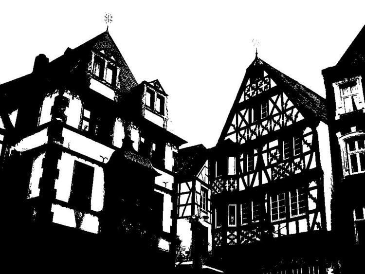
Variant 2

Result.

Limitations

Otsu’s method exhibits the relatively good performance if the histogram can be assumed to have bimodal distribution and assumed to possess a deep and sharp valley between two peaks. But if the object area is small compared with the background area, the histogram no longer exhibits bimodality. And if the variances of the object and the background intensities are large compared to the mean difference, or the image is severely corrupted by additive noise, the sharp valley of the gray level histogram is degraded. Then the possibly incorrect threshold determined by Otsu’s method results in the segmentation error. (Here we define the object size to be the ratio of the object area to the entire image area and the mean difference to be the difference of the average intensities of the object and the background)

From the experimental results, the performance of global thresholding techniques including Otsu’s method is shown to be limited by the small object size, the small mean difference, the large variances of the object and the background intensities, the large amount of noise added, and so on.

Improvements

There are many improvements focusing on different limitations for Otsu's method. One famous and effective way is known as two-dimensional Otsu's method. In this approach, the gray-level value of each pixel as well as the average value of its immediate neighborhood is studied so that the binarization results are greatly improved, especially for those images corrupted by noise.

At each pixel, the average gray-level value of the neighborhood is calculated. Let the gray level of a given picture be divided into L values and the average gray level is also divided into the same L values. Then a pair is formed: the pixel gray level and the average of the neighborhood. Each pair belongs to a 2-dimensional bin. The total number of bins is obviously L × L . The total number of occurrence(frequency), f i j , of a pair ( i , j ) divided by the total number of pixels in the image N , defines the joint probability mass function in 2-dimensional histogram:

P i j = f i j N , ∑ i = 0 L − 1 ∑ j = 0 L − 1 P i j = 1

And the 2-dimensional Otsu's method will be developed based on the 2-dimensional histogram as follows.

The probabilities of two classes can be denoted as:

ω 0 = ∑ i = 0 s − 1 ∑ j = 0 t − 1 P i j ω 1 = ∑ i = s L − 1 ∑ j = t L − 1 P i j

The intensity means value vectors of two classes and total mean vector can be expressed as follows:

μ 0 = [ μ 0 i , μ 0 j ] T = [ ∑ i = 0 s − 1 ∑ j = 0 t − 1 i P i j ω 0 , ∑ i = 0 s − 1 ∑ j = 0 t − 1 j P i j ω 0 ] T μ 1 = [ μ 1 i , μ 1 j ] T = [ ∑ i = s L − 1 ∑ j = t L − 1 i P i j ω 1 , ∑ i = s L − 1 ∑ j = t L − 1 j P i j ω 1 ] T μ T = [ μ T i , μ T j ] T = [ ∑ i = 0 L − 1 ∑ j = 0 L − 1 i P i j , ∑ i = 0 L − 1 ∑ j = 0 L − 1 j P i j ] T

In most cases, the probability off-diagonal will be negligible so it's easy to verify:

ω 0 + ω 1 ≅ 1 ω 0 μ 0 + ω 1 μ 1 ≅ μ T

The inter-class discrete matrix is defined as

S b = ∑ k = 0 1 ω k [ ( μ k − μ T ) ( μ k − μ T ) T ]

The trace of discrete matrix can be expressed as

tr ⁡ ( S b ) = ω 0 [ ( μ 0 i − μ T i ) 2 + ( μ 0 j − μ T j ) 2 ] + ω 1 [ ( μ 1 i − μ T i ) 2 + ( μ 1 j − μ T j ) 2 ] = ( μ T i ω 0 − μ i ) 2 + ( μ T j ω 0 − μ j ) 2 ω 0 ( 1 − ω 0 )

where

μ i = ∑ i = 0 s ∑ j = 0 t i P i j μ j = ∑ i = 0 s ∑ j = 0 t j P i j

Similar to one-dimensional Otsu's method, the optimal threshold ( s , t ) is obtained by maximizing tr ⁡ ( S b ) .

Algorithm

The s and t is obtained iteratively which is similar with one-dimensional Otsu's method. The values of s and t are changed till we obtain the maximum of tr ⁡ ( S b ) , that is

Notice that for evaluating tr ⁡ ( S b ) , we can use a fast recursive dynamic programming algorithm to improve time performance. However, even with the dynamic programming approach, 2d Otsu's method still has large time complexity. Therefore, many researches have been done to reduce the computation cost.

If summed area tables are used to build the 3 tables, sum over P_i_j, sum over i * P_i_j, and sum over j * P_i_j, then the runtime complexity is the maximum of (O(N_pixels), O(N_bins*N_bins)). Note that if only coarse resolution is needed in terms of threshold, N_bins can be reduced.

Matlab implementation

function inputs and output:

hists is a 256 × 256 2D-histogram of grayscale value and neighborhood average grayscale value pair.

total is the number of pairs in the given image.

threshold is the threshold obtained.

References

Otsu's method Wikipedia

(Text) CC BY-SA

Contents

Method

Algorithm

MATLAB implementation

Variant 1

Variant 2

Limitations

Improvements

Algorithm

Matlab implementation

References