Optimal stopping - Alchetron, The Free Social Encyclopedia

16 backward induction and optimal stopping times

In mathematics, the theory of optimal stopping or early stopping is concerned with the problem of choosing a time to take a particular action, in order to maximise an expected reward or minimise an expected cost. Optimal stopping problems can be found in areas of statistics, economics, and mathematical finance (related to the pricing of American options). A key example of an optimal stopping problem is the secretary problem. Optimal stopping problems can often be written in the form of a Bellman equation, and are therefore often solved using dynamic programming.

Discrete time case

Stopping rule problems are associated with two objects:

A sequence of random variables X 1 , X 2 , … , whose joint distribution is something assumed to be known
A sequence of 'reward' functions ( y i ) i ≥ 1 which depend on the observed values of the random variables in 1.: y i = y i ( x 1 , … , x i )

Given those objects, the problem is as follows:

You are observing the sequence of random variables, and at each step i , you can choose to either stop observing or continue

If you stop observing at step i , you will receive reward y i

You want to choose a stopping rule to maximise your expected reward (or equivalently, minimise your expected loss)

Continuous time case

Consider a gain processes G = ( G t ) t ≥ 0 defined on a filtered probability space ( Ω , F , ( F t ) t ≥ 0 , P ) and assume that G is adapted to the filtration. The optimal stopping problem is to find the stopping time τ ∗ which maximizes the expected gain

V t T = E G τ ∗ = sup t ≤ τ ≤ T E G τ

where V t T is called the value function. Here T can take value ∞ .

A more specific formulation is as follows. We consider an adapted strong Markov process X = ( X t ) t ≥ 0 defined on a filtered probability space ( Ω , F , ( F t ) t ≥ 0 , P x ) where P x denotes the probability measure where the stochastic process starts at x . Given continuous functions M , L , and K , the optimal stopping problem is

V ( x ) = sup 0 ≤ τ ≤ T E x ( M ( X τ ) + ∫ 0 τ L ( X t ) d t + sup 0 ≤ t ≤ τ K ( X t ) ) .

This is sometimes called the MLS (which stand for Mayer, Lagrange, and supremum, respectively) formulation.

Solution methods

There are generally two approaches of solving optimal stopping problems. When the underlying process (or the gain process) is described by its unconditional finite-dimensional distributions, the appropriate solution technique is the martingale approach, so called because it uses martingale theory, the most important concept being the Snell envelope. In the discrete time case, if the planning horizon T is finite, the problem can also be easily solved by dynamic programming.

When the underlying process is determined by a family of (conditional) transition functions leading to a Markov family of transition probabilities, powerful analytical tools provided by the theory of Markov processes can often be utilized and this approach is referred to as the Markov method. The solution is usually obtained by solving the associated free-boundary problems (Stefan problems).

A jump diffusion result

Let Y t be a Lévy diffusion in R k given by the SDE

d Y t = b ( Y t ) d t + σ ( Y t ) d B t + ∫ R k γ ( Y t − , z ) N ¯ ( d t , d z ) , Y 0 = y

where B is an m -dimensional Brownian motion, N ¯ is an l -dimensional compensated Poisson random measure, b : R k → R k , σ : R k → R k × m , and γ : R k × R k → R k × l are given functions such that a unique solution ( Y t ) exists. Let S ⊂ R k be an open set (the solvency region) and

τ S = inf { t > 0 : Y t ∉ S }

be the bankruptcy time. The optimal stopping problem is:

V ( y ) = sup τ ≤ τ S J τ ( y ) = sup τ ≤ τ S E y [ M ( Y τ ) + ∫ 0 τ L ( Y t ) d t ] .

It turns out that under some regularity conditions, the following verification theorem holds:

If a function ϕ : S ¯ → R satisfies

ϕ ∈ C ( S ¯ ) ∩ C 1 ( S ) ∩ C 2 ( S ∖ ∂ D ) where the continuation region is D = { y ∈ S : ϕ ( y ) > M ( y ) } ,

ϕ ≥ M on S , and

A ϕ + L ≤ 0 on S ∖ ∂ D , where A is the infinitesimal generator of ( Y t )

then ϕ ( y ) ≥ V ( y ) for all y ∈ S ¯ . Moreover, if

A ϕ + L = 0 on D

Then ϕ ( y ) = V ( y ) for all y ∈ S ¯ and τ ∗ = inf { t > 0 : Y t ∉ D } is an optimal stopping time.

These conditions can also be written is a more compact form (the integro-variational inequality):

max { A ϕ + L , M − ϕ } = 0 on S ∖ ∂ D .

Coin tossing

(Example where E ( y i ) converges)

You have a fair coin and are repeatedly tossing it. Each time, before it is tossed, you can choose to stop tossing it and get paid (in dollars, say) the average number of heads observed.

You wish to maximise the amount you get paid by choosing a stopping rule. If X_i (for i ≥ 1) forms a sequence of independent, identically distributed random variables with Bernoulli distribution

Bern ( 1 2 ) ,

and if

y i = 1 i ∑ k = 1 i X k

then the sequences ( X i ) i ≥ 1 , and ( y i ) i ≥ 1 are the objects associated with this problem.

House selling

(Example where E ( y i ) does not necessarily converge)

You have a house and wish to sell it. Each day you are offered X n for your house, and pay k to continue advertising it. If you sell your house on day n , you will earn y n , where y n = ( X n − n k ) .

You wish to maximise the amount you earn by choosing a stopping rule.

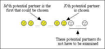
In this example, the sequence ( X i ) is the sequence of offers for your house, and the sequence of reward functions is how much you will earn.

Secretary problem

(Example where ( X i ) is a finite sequence)

You are observing a sequence of objects which can be ranked from best to worst. You wish to choose a stopping rule which maximises your chance of picking the best object.

Here, if R 1 , … , R n (n is some large number, perhaps) are the ranks of the objects, and y i is the chance you pick the best object if you stop intentionally rejecting objects at step i, then ( R i ) and ( y i ) are the sequences associated with this problem. This problem was solved in the early 1960s by several people. An elegant solution to the secretary problem and several modifications of this problem is provided by the more recent odds algorithm of optimal stopping (Bruss algorithm).

Search theory

Economists have studied a number of optimal stopping problems similar to the 'secretary problem', and typically call this type of analysis 'search theory'. Search theory has especially focused on a worker's search for a high-wage job, or a consumer's search for a low-priced good.

Option trading

In the trading of options on financial markets, the holder of an American option is allowed to exercise the right to buy (or sell) the underlying asset at a predetermined price at any time before or at the expiry date. Therefore, the valuation of American options is essentially an optimal stopping problem. Consider a classical Black-Scholes set-up and let r be the risk-free interest rate and δ and σ be the dividend rate and volatility of the stock. The stock price S follows geometric Brownian motion

S t = S 0 exp ⁡ { ( r − δ − σ 2 2 ) t + σ B t }

under the risk-neutral measure.

When the option is perpetual, the optimal stopping problem is

V ( x ) = sup τ E x [ e − r τ g ( S τ ) ]

where the payoff function is g ( x ) = ( x − K ) + for a call option and g ( x ) = ( K − x ) + for a put option. The variational inequality is

max { 1 2 σ 2 x 2 V ″ ( x ) + ( r − δ ) x V ′ ( x ) − r V ( x ) , g ( x ) − V ( x ) } = 0

for all x ∈ ( 0 , ∞ ) ∖ { b } where b is the exercise boundary. The solution is known to be

(Perpetual call) V ( x ) = { ( b − K ) ( x / b ) γ x ∈ ( 0 , b ) x − K x ∈ [ b , ∞ ) where γ = ( ν 2 + 2 r − ν ) / σ and ν = ( r − δ ) / σ − σ / 2 , b = γ K / ( γ − 1 ) .

(Perpetual put) V ( x ) = { K − x x ∈ ( 0 , c ] ( K − c ) ( x / c ) γ ~ x ∈ ( c , ∞ ) where γ ~ = − ( ν 2 + 2 r + ν ) / σ and ν = ( r − δ ) / σ − σ / 2 , c = γ ~ K / ( γ ~ − 1 ) .

On the other hand, when the expiry date is finite, the problem is associated with a 2-dimensional free-boundary problem with no known closed-form solution. Various numerical methods can however be used. See Black–Scholes model #American options for various valuation methods here, as well as Fugit for a discrete, tree based, calculation of the optimal time to exercise.

References

Optimal stopping Wikipedia

(Text) CC BY-SA