One way analysis of variance

Assumptions

The results of a one-way ANOVA can be considered reliable as long as the following assumptions are met:

Response variable residuals are normally distributed (or approximately normally distribution).

Variances of populations are equal.

Responses for a given group are independent and identically distributed normal random variables (not a simple random sample (SRS)).

If data are ordinal, a non-parametric alternative to this test should be used such as Kruskal–Wallis one-way analysis of variance. If the variances are not known to be equal, a generalization of 2-sample Welch's t-test can be used.

Departures from population normality

ANOVA is a relatively robust procedure with respect to violations of the normality assumption.

The one-way ANOVA can be generalized to the factorial and multivariate layouts, as well as to the analysis of covariance.

It is often stated in popular literature that none of these F-tests are robust when there are severe violations of the assumption that each population follows the normal distribution, particularly for small alpha levels and unbalanced layouts. Furthermore, it is also claimed that if the underlying assumption of homoscedasticity is violated, the Type I error properties degenerate much more severely.

However, this is a misconception, based on work done in the 1950s and earlier. The first comprehensive investigation of the issue by Monte Carlo simulation was Donaldson (1966). He showed that under the usual departures (positive skew, unequal variances) "the F-test is conservative" so is less likely than it should be to find that a variable is significant. However, as either the sample size or the number of cells increases, "the power curves seem to converge to that based on the normal distribution". Tiku (1971) found that "the non-normal theory power of F is found to differ from the normal theory power by a correction term which decreases sharply with increasing sample size." The problem of non-normality, especially in large samples, is far less serious than popular articles would suggest.

The current view is that "Monte-Carlo studies were used extensively with normal distribution-based tests to determine how sensitive they are to violations of the assumption of normal distribution of the analyzed variables in the population. The general conclusion from these studies is that the consequences of such violations are less severe than previously thought. Although these conclusions should not entirely discourage anyone from being concerned about the normality assumption, they have increased the overall popularity of the distribution-dependent statistical tests in all areas of research."

For nonparametric alternatives in the factorial layout, see Sawilowsky. For more discussion see ANOVA on ranks.

The model

The normal linear model describes treatment groups with probability distributions which are identically bell-shaped (normal) curves with different means. Thus fitting the models requires only the means of each treatment group and a variance calculation (an average variance within the treatment groups is used). Calculations of the means and the variance are performed as part of the hypothesis test.

The commonly used normal linear models for a completely randomized experiment are:

y i , j = μ j + ε i , j (the means model)

or

y i , j = μ + τ j + ε i , j (the effects model)

where

i = 1 , … , I is an index over experimental units j = 1 , … , J is an index over treatment groups I j is the number of experimental units in the jth treatment group I = ∑ j I j is the total number of experimental units y i , j are observations μ j is the mean of the observations for the jth treatment group μ is the grand mean of the observations τ j is the jth treatment effect, a deviation from the grand mean ∑ τ j = 0 μ j = μ + τ j ε ∼ N ( 0 , σ 2 ) , ε i , j are normally distributed zero-mean random errors.

The index i over the experimental units can be interpreted several ways. In some experiments, the same experimental unit is subject to a range of treatments; i may point to a particular unit. In others, each treatment group has a distinct set of experimental units; i may simply be an index into the j t h list.

The data and statistical summaries of the data

One form of organizing experimental observations y i j is with groups in columns:

Comparing model to summaries: μ = m and μ j = m j . The grand mean and grand variance are computed from the grand sums, not from group means and variances.

The hypothesis test

Given the summary statistics, the calculations of the hypothesis test are shown in tabular form. While two columns of SS are shown for their explanatory value, only one column is required to display results.

M S E r r o r is the estimate of variance corresponding to σ 2 of the model.

Analysis summary

The core ANOVA analysis consists of a series of calculations. The data is collected in tabular form. Then

Each treatment group is summarized by the number of experimental units, two sums, a mean and a variance. The treatment group summaries are combined to provide totals for the number of units and the sums. The grand mean and grand variance are computed from the grand sums. The treatment and grand means are used in the model.

The three DFs and SSs are calculated from the summaries. Then the MSs are calculated and a ratio determines F.

A computer typically determines a p-value from F which determines whether treatments produce significantly different results. If the result is significant, then the model provisionally has validity.

If the experiment is balanced, all of the I j terms are equal so the SS equations simplify.

In a more complex experiment, where the experimental units (or environmental effects) are not homogeneous, row statistics are also used in the analysis. The model includes terms dependent on i . Determining the extra terms reduces the number of degrees of freedom available.

Example

Consider an experiment to study the effect of three different levels of a factor on a response (e.g. three levels of a fertilizer on plant growth). If we had 6 observations for each level, we could write the outcome of the experiment in a table like this, where a₁, a₂, and a₃ are the three levels of the factor being studied.

The null hypothesis, denoted H₀, for the overall F-test for this experiment would be that all three levels of the factor produce the same response, on average. To calculate the F-ratio:

Step 1: Calculate the mean within each group:

Y ¯ 1 = 1 6 ∑ Y 1 i = 6 + 8 + 4 + 5 + 3 + 4 6 = 5 Y ¯ 2 = 1 6 ∑ Y 2 i = 8 + 12 + 9 + 11 + 6 + 8 6 = 9 Y ¯ 3 = 1 6 ∑ Y 3 i = 13 + 9 + 11 + 8 + 7 + 12 6 = 10

Step 2: Calculate the overall mean:

Y ¯ = ∑ i Y ¯ i a = Y ¯ 1 + Y ¯ 2 + Y ¯ 3 a = 5 + 9 + 10 3 = 8 where a is the number of groups.

Step 3: Calculate the "between-group" sum of squared differences:

S B = n ( Y ¯ 1 − Y ¯ ) 2 + n ( Y ¯ 2 − Y ¯ ) 2 + n ( Y ¯ 3 − Y ¯ ) 2 = 6 ( 5 − 8 ) 2 + 6 ( 9 − 8 ) 2 + 6 ( 10 − 8 ) 2 = 84

where n is the number of data values per group.

The between-group degrees of freedom is one less than the number of groups

f b = 3 − 1 = 2

so the between-group mean square value is

M S B = 84 / 2 = 42

Step 4: Calculate the "within-group" sum of squares. Begin by centering the data in each group

The within-group sum of squares is the sum of squares of all 18 values in this table

S W = ( 1 ) 2 + ( 3 ) 2 + ( − 1 ) 2 + ( 0 ) 2 + ( − 2 ) 2 + ( − 1 ) 2 + ( − 1 ) 2 + ( 3 ) 2 + ( 0 ) 2 + ( 2 ) 2 + ( − 3 ) 2 + ( − 1 ) 2 + ( 3 ) 2 + ( − 1 ) 2 + ( 1 ) 2 + ( − 2 ) 2 + ( − 3 ) 2 + ( 2 ) 2 =   1 + 9 + 1 + 0 + 4 + 1 + 1 + 9 + 0 + 4 + 9 + 1 + 9 + 1 + 1 + 4 + 9 + 4 =   68

The within-group degrees of freedom is

f W = a ( n − 1 ) = 3 ( 6 − 1 ) = 15

Thus the within-group mean square value is

M S W = S W / f W = 68 / 15 ≈ 4.5

Step 5: The F-ratio is

F = M S B M S W ≈ 42 / 4.5 ≈ 9.3

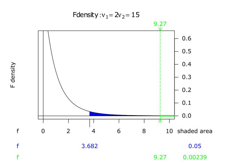
The critical value is the number that the test statistic must exceed to reject the test. In this case, F_crit(2,15) = 3.68 at α = 0.05. Since F=9.3 > 3.68, the results are significant at the 5% significance level. One would reject the null hypothesis, concluding that there is strong evidence that the expected values in the three groups differ. The p-value for this test is 0.002.

After performing the F-test, it is common to carry out some "post-hoc" analysis of the group means. In this case, the first two group means differ by 4 units, the first and third group means differ by 5 units, and the second and third group means differ by only 1 unit. The standard error of each of these differences is 4.5 / 6 + 4.5 / 6 = 1.2 . Thus the first group is strongly different from the other groups, as the mean difference is more times the standard error, so we can be highly confident that the population mean of the first group differs from the population means of the other groups. However, there is no evidence that the second and third groups have different population means from each other, as their mean difference of one unit is comparable to the standard error.

Note F(x, y) denotes an F-distribution cumulative distribution function with x degrees of freedom in the numerator and y degrees of freedom in the denominator.