Oblivious data structure

Oblivious RAM

Goldreich and Ostrovsky proposed this term on software protection.

The memory access of oblivious RAM is probabilistic and the probabilistic distribution is independent of the input. In the paper composed by Goldreich and Ostrovsky have theorem to oblivious RAM: Let RAM(m) denote a RAM with m memory locations and access to a random oracle machine. Then t steps of an arbitrary RAM(m) program can be simulated by less than O ( t ( log 2 ⁡ t ) 3 ) steps of an oblivious R A M ( m ( log 2 ⁡ m ) 2 ) . Every oblivious simulation of RAM(m) must make at least max { m , ( t − 1 ) log 2 ⁡ m } accesses in order to simulate t steps.

Now we have the square-root algorithm to simulate the oblivious ram working.

1. For each m accesses, randomly permute first m + m memory.
2. Check the shelter words first if we want to access a word.
3. If the word is there, access one of the dummy words. And if the word is not there, find the permuted location.

To access original RAM in t steps we need to simulate it with t + m steps for the oblivious RAM. For each access, the cost would be O( m ⋅ log ⁡ m ).

Another way to simulate is hierarchical algorithm. The basic idea is to consider the shelter memory as a buffer, and extend it to the multiple levels of buffers. For level I, there are 4 i buckets and for each bucket has log t items. For each level there is a random selected hash function.

The operation is like the following: At first load program to the last level, which can be say has 4 t buckets. For reading, check the bucket h i ( V ) from each level, If (V,X) is already found, pick a bucket randomly to access, and if it is not found, check the bucket h i ( V ) , there is only one real match and remaining are dummy entries . For writing, put (V,X) to the first level, and if the first I levels are full, move all I levels to I + 1 levels and empty the first I levels.

The time cost for each level cost O(log t); cost for every access is O ( ( log ⁡ t ) 2 ) ; The cost of Hashing is O ( t ( log ⁡ t ) 3 ) .

Oblivious Tree

An Oblivious Tree is a rooted tree with the following property:

All the leaves are in the same level.

All the internal nodes have degree at most 3.

Only the nodes along the rightmost path in the tree may have degree of one.

The oblivious tree is a data structure similar to 2-3 Tree, but with the additional property of being oblivious. The rightmost path may have degree one and this can help to describe the update algorithms. Oblivious tree requires randomization to achieve a O ( log ⁡ ( n ) ) running time for the update operations. And for two sequences of operations M and N acting to the tree, the output of the tree has the same output probability distributions. For the tree, there are three operations:

CREATE (L)

build a new tree storing the sequence of values L at its leaves.

INSERT (b, i,T)

insert a new leaf node storing the value b as the i^th leaf of the tree T.

DELETE (i, T)

remove the i^th leaf from T.

Step of Create: The list of nodes at the i^thlevel is obtained traversing the list of nodes at level i+1 from left to right and repeatedly doing the following:

1. Choose d {2, 3} uniformly at random.
2. If there are less than d nodes left at level i+1, set d equal to the number of nodes left.
3. Create a new node n at level I with the next d nodes at level i+1 as children and compute the size of n as the sum of the sizes of its children.

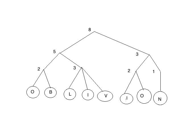
For example, if the coin tosses of d {2, 3} has an outcome of: 2, 3, 2, 2, 2, 2, 3 stores the string “OBLIVION” as follow oblivious tree.

Both the INSERT (b, I, T) and DELETE(I, T) have the O(log n) expected running time. And for INSERT and DELETE we have:

INSERT (b, I, CREATE (L)) = CREATE (L [1] + …….., L[ i], b, L[i+1]………..) DELETE (I, CREATE (L)) = CREATE (L[1]+ ………L[I - 1], L[i+1], ………..)

For example, if the CREATE (ABCDEFG) or INSERT (C, 2, CREATE (ABDEFG)) is run, it yields the same probabilities of out come between these two operations.

Cache-Oblivious kd-tree

A kd-tree is used for answering the orthogonal range queries.

The kd-tree is a binary tree of height O(log₂N) with the N points into two subsets of equal size. On even levels of the tree the dividing lines are horizontal, and on odd levels of the tree the dividing lines are vertical. In this way rectangular region is associated with each node, and the nodes on any particular level of the tree partition the plane into disjoint regions. This structure answers queries in O(log_B N+ T/B)memory transfers using O(N log₂²N) space.

In the RAM model, a kd-tree on N points can be constructed in recursion in O (Nlog₂N) times; the root dividing line is found using an O(N) time median algorithm, the points are distributed into two sets according to this line in O(N) time, and the two sub trees are constructed recursively.

Cache-Oblivious Buffer Heap

Cache-oblivious buffer heap is a cache-oblivious priority queue that supports Delete, Delete-Min and Decrease-Key operation in O(1/B(log N/M)) (B is the size of a block; N is the number of items in the priority queue; M is the items in the memory) amortized cache-misses each. A buffer heap with N items consists of 1+log₂N levels.

Delete (x) operation deletes element x from queue if it exists.

Delete-Min () operation retrieves and deletes an element with the minimum key from the queue if it exists.

A Decrease-Key (x, k_x) operation inserts the element x with the key k_x into the queue if x does not already exist in the queue, other wise it replaces the smallest key k’_x of x in the queue with k_x provided k_x < k’_x, and deletes all the remaining keys of x in the queue.

Application of Buffer Heap:

Cache-oblivious Undirected single source shortest path problem (SSSP): The algorithm incurs O(m/B(log₂ n/M)) cache-misses for the O(m) priority queue operations it performs. In addition to that it incurs O(n +m/B) cache-misses for accessing O(n) adjacency lists.

Cache-oblivious Directed SSSP

Cache-aware Undirected APSP

Cache Oblivious Binary Search Tree

This data structure has a cache oblivious layout of static binary search trees permitting searches in the asymptotically optimal number of memory transfers. This data structure has an advantage is avoiding usage of the pointer. The basic idea of this data structure is to maintain a dynamic binary tree of height log n + O(1) using existing methods, embed this tree in a static binary tree.

The depth d(v) of a node v in a tree T is the number of nodes on the simple path from the node to the root. The height h(T) of T is the maximum depth of a node in T, and the size |T| of T is the number of nodes in T. A complete tree T is a tree with 2^h(T)-1 nodes.

There are four memory layouts for static trees: DFS, inorder, BFS and van Emde Boas tree layouts.

DFS layout: The nodes of T are stored in the order they are visited by a left-to-right depth first traversal of T.

Inorder layout: The nodes of T are stored in the order that they are visited by a left-to-right inorder traversal of T.

BFS layout: The nodes of T are stored in the order they are visited by a left-to-right breath first traversal of T.

Van Emde Boas layout: The layout is defined recursively. A tree with only one node is a single node record. If a tree T has two or more nodes, let H₀=h(T)/2, let T₀ be the tree consisting of all nodes in T with depth at most H₀, and let T₁,……., T_k be the subtrees of T rooted at nodes with depth H₀+1, numbered from left to right. We denote T₀ the top tree and T₁,……., T_k the bottom trees of the recursion_.

Using the structure to sort n elements, it uses (1 +ε )n times the element size of memory, and performs searches in worst case O(log_Bn) memory transfers, updates in amortized O((log² n)= (εB)) memory transfers, and range queries in worst case O(log_B n+ k=B) memory transfers, where k is the size of the output.

Quickheaps

Qickheap is a simple and efficient data structure for implementing priority queue in main memory and secondary memory. Quickheaps enable efficient element insertion, minimum extraction, deletion of arbitrary elements and modification of the priority of elements within the heap. For a queue has m elements, it requires O(log m) extra integers.

To implement a quickheap we need these structures:

An array heap to store elements.

A stack S to store the positions of pivots partitioning heap.

An integer idx to indicate the first cell of the quickheap.

An integer capacity to indicate the size of heap.

The Quick Operations include:

Creation of Empty Quickheaps;

Quick-heapifying an Array;

Finding the Minimum;

Extraction the Minimum;

Inserting Elements;

Cache-Oblivious Priority Queue

The cache-oblivious priority queue can implement operations including insertion, deletion and delete-min in O(1/B(log_M/B N/B)) amortized memory transfers(M and B are memory and block transfer size).

The priority queue containing N elements consists of θ (loglogN₀) levels whose sizes vary from N₀= θ (N) to some small size c beneath a constant threshold c_t. A level stores elements in a number of buffers, which are also used to transfer elements between levels. The queue is stored in a liner array. The levels are stored consecutively from smallest to largest with each level occupying a single region of memory.

Operations:

Push: Insert x elements into level X^3/2. Time O(X+ X^1/2)

Pull: removes and returns the X elements with the smallest keys from level X^3/2.Time O(X log₂X)+ O(X)

Delete-Min: Time O(log₂N)

Delete: O(log₂N)

Funnels

A K-funnel is a complete binary tree with K leaves, stored according to the van Emde Boas layout. Each of the recursive subtrees of a K-funnel is a K -funnel. In addition to the nodes, edges in a K-funnel store buffers. The buffers can be stored in an arbitrary order along with the recursive subtrees.

For a K-funnel occupies θ(K²) storage, and at least K² storage. If the input lists have K³ elements total, then a K-funnel fills the output buffer in O(K³/B(log_M/B K³/B)+K) memory transfers.

And also there is a funnel heap data structure. The funnel heap is composed of a sequence of doubly exponentially increasing size. There is a delete-min operation for this data structure and the operation is straightforward: it extracts the first element from the first buffer, recursively filling it if it was empty.

Application of Oblivious Data Structure

In algorithm we have the problem of Breadth-first search (BFS) and the single-source shortest path (SSSP), and these two problems are well understood in the RAM model, where the cost of a memory access is assumed to be independent of the accessed memory location. But modern computers contain a hierarchy of memory levels, and the cost of a memory access depends on the currently lowest memory level that contains the accessed element.

Cache-Oblivious Breadth-First Search

First the algorithm constructs the data structure. In the beginning, we need to build a spanning tree for G and then construct an Euler tour T for the tree (can use the Prim algorithm). Then assign to each node v the rank in T of the first occurrence of v, and denote this value r(v).

The data structure consists of h levels G₁, …. ,G_h where each level stores a subset of the adjacency lists of the graph G. Each adjacency list N(v) appears in exactly one of the levels unless it has been removed from the structure.

Initially, all adjacency lists are in level h. Over time the query procedure GETEDGELISTS moves the adjacency list of each node from higher numbered to lower numbered levels, until the adjacency list finally reaches level G₁ and is removed. The pseudo code is as following.

GETEDGELISTS (S,i) 1 S’’← {v∈S | N(v) is not stored in level Gi} 2 if S’’ ≠ ∮: 3 X← GETEDGELISTS (S’, i+1) 4 for each gi-edge-group g in X 5 insert g in Gi 6 for each gi-1– edge-group r in Gi containing N(v) for some v ∈ S 7 remove r from Gi 8 include r in the output set

The cost of constructing the initial spanning tree is O(ST(E)); the Eular tour can be constructed in O(Sort(V)) I/Os. Assigning ranks to nodes and labeling the edges with the assigned ranks requires further O(Sort(E)) I/Os. The total preprocessing of the data structure costs O(ST(E)+ Sort(E)) I/Os.

Kumar and Schwabe’s SSSP algorithm

Kumar and Schwabe’s algorithm is a variant of Dijkstra’s algorithm. It solves the SSSP problem in O(n+ (m/B) log₂(n/B)) memory transfers. And this algorithm uses a priority queue supporting the UPDATE() operation.

This algorithm is different from Dijkstra’s algorithm. When a vertice w ∈ V is visited, for each neighbor v of w the algorithm performs an UPDATE(v, d(w) + l(vw)) operation on the priority queue Q. An UPDATE(v, p) operation inserts element v in Q with priority p if v is not already present in Q; otherwise, if v is already present in Q with priority p’, the priority of v is changed to min(p, p’).

The I/O complexity of Kumar and Schwabe’s algorithm is O(n +(m/B) log₂(n/B)).