Nonlinear conjugate gradient method

In numerical optimization, the nonlinear conjugate gradient method generalizes the conjugate gradient method to nonlinear optimization. For a quadratic function f ( x ) :

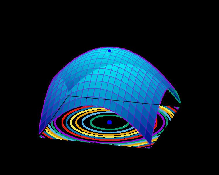
The minimum of f is obtained when the gradient is 0:

Whereas linear conjugate gradient seeks a solution to the linear equation A T A x = A T b , the nonlinear conjugate gradient method is generally used to find the local minimum of a nonlinear function using its gradient ∇ x f alone. It works when the function is approximately quadratic near the minimum, which is the case when the function is twice differentiable at the minimum and the second derivative is non-singular there.

Given a function f ( x ) of N variables to minimize, its gradient ∇ x f indicates the direction of maximum increase. One simply starts in the opposite (steepest descent) direction:

with an adjustable step length α and performs a line search in this direction until it reaches the minimum of f :

After this first iteration in the steepest direction Δ x 0 , the following steps constitute one iteration of moving along a subsequent conjugate direction s n , where s 0 = Δ x 0 :

1. Calculate the steepest direction: Δ x n = − ∇ x f ( x n ) ,
2. Compute β n according to one of the formulas below,
3. Update the conjugate direction: s n = Δ x n + β n s n − 1
4. Perform a line search: optimize α n = arg ⁡ min α f ( x n + α s n ) ,
5. Update the position: x n + 1 = x n + α n s n ,

With a pure quadratic function the minimum is reached within N iterations (excepting roundoff error), but a non-quadratic function will make slower progress. Subsequent search directions lose conjugacy requiring the search direction to be reset to the steepest descent direction at least every N iterations, or sooner if progress stops. However, resetting every iteration turns the method into steepest descent. The algorithm stops when it finds the minimum, determined when no progress is made after a direction reset (i.e. in the steepest descent direction), or when some tolerance criterion is reached.

Within a linear approximation, the parameters α and β are the same as in the linear conjugate gradient method but have been obtained with line searches. The conjugate gradient method can follow narrow (ill-conditioned) valleys, where the steepest descent method slows down and follows a criss-cross pattern.

Four of the best known formulas for β n are named after their developers:

These formulas are equivalent for a quadratic function, but for nonlinear optimization the preferred formula is a matter of heuristics or taste. A popular choice is β = max { 0 , β P R } , which provides a direction reset automatically.

Newton-based methods – Newton-Raphson Algorithm, Quasi-Newton methods (e.g., BFGS method) – tend to converge in fewer iterations, although each iteration typically requires more computation than a conjugate gradient iteration, as Newton-like methods require computing the Hessian (matrix of second derivatives) in addition to the gradient. Quasi-Newton methods also require more memory to operate (see also the limited-memory L-BFGS method).