Nanoindentation

Background

In a traditional indentation test (macro or micro indentation), a hard tip whose mechanical properties are known (frequently made of a very hard material like diamond) is pressed into a sample whose properties are unknown. The load placed on the indenter tip is increased as the tip penetrates further into the specimen and soon reaches a user-defined value. At this point, the load may be held constant for a period or removed. The area of the residual indentation in the sample is measured and the hardness, H , is defined as the maximum load, P m a x , divided by the residual indentation area, A r :

For most techniques, the projected area may be measured directly using light microscopy. As can be seen from this equation, a given load will make a smaller indent in a "hard" material than a "soft" one.

This technique is limited due to large and varied tip shapes, with indenter rigs which do not have very good spatial resolution (the location of the area to be indented is very hard to specify accurately). Comparison across experiments, typically done in different laboratories, is difficult and often meaningless. Nanoindentation improves on these macro- and micro-indentation tests by indenting on the nanoscale with a very precise tip shape, high spatial resolutions to place the indents, and by providing real-time load-displacement (into the surface) data while the indentation is in progress.

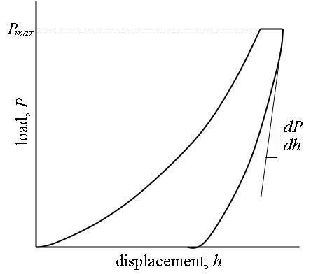
In nanoindentation small loads and tip sizes are used, so the indentation area may only be a few square micrometres or even nanometres. This presents problems in determining the hardness, as the contact area is not easily found. Atomic force microscopy or scanning electron microscopy techniques may be utilized to image the indentation, but can be quite cumbersome. Instead, an indenter with a geometry known to high precision (usually a Berkovich tip, which has a three-sided pyramid geometry) is employed. During the course of the instrumented indentation process, a record of the depth of penetration is made, and then the area of the indent is determined using the known geometry of the indentation tip. While indenting, various parameters such as load and depth of penetration can be measured. A record of these values can be plotted on a graph to create a load-displacement curve (such as the one shown in Figure 1). These curves can be used to extract mechanical properties of the material.

E r = 1 β π 2 S A p ( h c ) ,

Where A p ( h c ) is the projected area of the indentation at the contact depth h c , and β is a geometrical constant on the order of unity. A p ( h c ) is often approximated by a fitting polynomial as shown below for a Berkovich tip:

A p ( h c ) = C 0 h c 2 + C 1 h c 1 + C 2 h c 1 / 2 + C 3 h c 1 / 4 + … + C 8 h c 1 / 128

Where C 0 for a Berkovich tip is 24.5 while for a cube corner (90°) tip is 2.598. The reduced modulus E r is related to Young's modulus E s of the test specimen through the following relationship from contact mechanics:

1 / E r = ( 1 − ν i 2 ) / E i + ( 1 − ν s 2 ) / E s .

Here, the subscript i indicates a property of the indenter material and ν is Poisson's ratio. For a diamond indenter tip, E i is 1140 GPa and ν i is 0.07. Poisson’s ratio of the specimen, ν s , generally varies between 0 and 0.5 for most materials (though it can be negative) and is typically around 0.3.

H = P m a x A r .

The hardness is given by the equation above, relating the maximum load to the indentation area. The area can be measured after the indentation by in-situ atomic force microscopy, or by 'after-the event' optical (or electron) microscopy. An example indentation image, from which the area may be determined, is shown at right.

Some nanoindenters use an area function based on the geometry of the tip, compensating for elastic load during the test. Use of this area function provides a method of gaining real-time nanohardness values from a load-displacement graph. However, there is some controversy over the use of area functions to estimate the residual areas versus direct measurement. An area function A p ( h c ) typically describes the projected area of an indent as a 2nd-order polynomial function of the indenter depth h . When too many coefficients are used, the function will begin to fit to the noise in the data, and inflection points will develop. If the curve can fit well with only two coefficients, this is the best. However, if many data points are used, sometimes all 6 coefficients will need to be used to get a good area function. Typically, 3 or 4 coefficients works well. Exclusive application of an area function in the absence of adequate knowledge of material response can lead to misinterpretation of resulting data. Cross-checking of areas microscopically is to be encouraged.

m = ∂ ln ⁡ σ ∂ ln ⁡ ε ˙ ,

where σ = σ ( ε ˙ ) is the flow stress and ε ˙ is the strain rate produced under the indenter. For nanoindentation experiments which include a holding period at constant load (i.e. the flat, top area of the load-displacement curve), m can be determined from

d ln ⁡ H = m d ln ⁡ ε p ˙ + n d ln ⁡ h p .

The subscripts p indicate these values are to be determined from the plastic components only.

V ∗ = 9 k B T ∂ ln ⁡ ε ˙ ∂ H ,

where T is the temperature and k_B is Boltzmann's constant. From the definition of m , it is easy to see that V ∗ ∝ ( H m ) − 1 .

Software

The indentation curves have often at least thousands of data points. The hardness and elastic modulus can quickly be calculated by using a programming language or a spreadsheet. Instrumented indentation testing machines come with the software specifically designed to analyze the indentation data from their own machine. The Indentation Grapher (Dureza) software is able to import text data from several commercial machines or custom made equipment. Spreadsheet programs such as MS-Excel or OpenOffice Calculate do not have the ability to fit to the non-linear power law equation from indentation data. A linear fit can be done by offset ( − h ( P 0 ) ) displacement so that the data passes through the origin. Then select the power law equation from the graphing X Y options.

The Martens hardness, H M , is a simple software for any programmer having minimal background to develop. The software starts by searching for the maximum displacement, h m a x , point and maximum load, P m a x .

H M = P m a x A s .

The displacement is used to calculate the contact surface area, A s , based on the indenter geometry. For a perfect Berkovich indenter the relationship is A s = 24.5 h m a x 2 .

The indentation hardness, H I T is defined slightly different.

H I T = P m a x A p .

Here, the hardness is related to the projected contact area A p .

As the indent size decreases the error caused by tip rounding increases. The tip wear can be accounted for within the software by using a simple polynomial function. As the indenter tip wears the C 1 value will increase. The user enters the values for C 0 and C 1 based on direct measurements such as SEM or AFM images of the indenter tip or indirectly by using a material of known elastic modulus or an atomic force microscope (AFM) image of an indentation.

A p = C 0 h m a x 2 + C 1 h m a x .

Calculating the elastic modulus with software involves using software filtering techniques to separate the critical unloading data from the rest of the load-displacement data. The start and end points are usually found by using user defined percentages. This user input increases the variability because of possible human error. It would be best if the entire calculation process was automatically done for more consistent results. A good nanoindentation machine prints out the load unload curve data with labels to each of the segments such as loading, top hold, unload, bottom hold, and reloading. If multiple cycles are used then each one should be labeled. However mores nanoindenters only give the raw data for the load-unload curves. An automatic software technique finds the sharp change from the top hold time to the beginning of the unloading. This can be found by doing a linear fit to the top hold time data. The unload data starts when the load is 1.5 times standard deviation less than the hold time load. The minimum data point is the end of the unloading data. The computer calculates the elastic modulus with this data according to the Oliver-Pharr (nonlinear). The Doerner-Nix method is less complicated to program because it is a linear curve fit of the selected minimum to maximum data. However, it is limited because the calculated elastic modulus will decrease as more data points are used along the unloading curve. The Oliver-Pharr nonlinear curve fit method to the unloading curve data where h is the depth variable, h f is the final depth and k and m are constants and coefficients. The software must use a nonlinear convergence method to solve for k , h f and m that best fits the unloading data. The slope is calculated by differentiating d P / d h at the maximum displacement.

P = k ( h − h f ) m .

An image of the indent can also be measured using software. The atomic force microscope (AFM) scans the indent. First the lowest point of the indentation is found. Make an array of lines around the using linear lines from indent center along the indent surface. Where the section line is more than several standard deviations (>3 σ ) from the surface noise the outline point is created. Then connect all of the outline points to build the entire indent outline. This outline will automatically include the pile-up contact area.

For nanoindentation experiments performed with a conical indenter on a thin film deposited on a substrate or on a multilayer sample, the NIMS Matlab toolbox is useful for load-displacement curves analysis and calculations of Young's modulus and hardness of the coating.

Devices

The construction of a depth-sensing indentation system is made possible by the inclusion of very sensitive displacement and load sensing systems. Load transducers must be capable of measuring forces in the micronewton range and displacement sensors are very frequently capable of sub-nanometer resolution. Environmental isolation is crucial to the operation of the instrument. Vibrations transmitted to the device, fluctuations in atmospheric temperature and pressure, and thermal fluctuations of the components during the course of an experiment can cause significant errors.

The ability to conduct nanoindentation studies with nanometer depth, and sub-nanonewton force resolution is also possible using a standard AFM setup. The AFM allows for nanomechanical studies to be conducted alongside topographic analyses, without the use of dedicated instruments. Load-displacement curves can be collected similarly for a variety of materials, and mechanical properties can be directly calculated from these curves.

Applications

Nanoindentation is a robust technique for determination of thin film properties for which conventional testing are not feasible. Conventional mechanical testing such as tensile testing or dynamic mechanical analysis (DMA) can only return the average property without any indication of variability across the sample. However, nanoindentation can be used for determination of local properties of homogeneous as well as heterogeneous materials.

Limitations

Conventional nanoindentation methods for calculation of Modulus of elasticity (based on the unloading curve) are limited to linear, isotropic materials.

Piles up and Sink in

Problems associated with the "pile-up" or "sink-in" of the material on the edges of the indent during the indentation process remain a problem that is still under investigation. It is possible to measure the pile-up contact area using computerized image analysis of atomic force microscope (AFM) images of the indentations. This process also depends on the linear isotropic elastic recovery for the indent reconstruction.

Nanoindentation on soft material

Nanoindentation of soft material has intrinsic challenges due to adhesion, surface detection and tip dependency of results. There is an ongoing research to overcome such problems.

Tip Dependency

While nanoindentation testing can be relatively simple, the interpretation of results is challenging. One of the main challenges is the use of proper tip depending on the application and proper interpretation of the results. For instance, it has been shown that the elastic modulus can be tip dependent