Neha Patil (Editor)

N curve

Updated on
Edit
Like
Comment
Share on FacebookTweet on TwitterShare on LinkedInShare on Reddit
N-curve

We take the functional theoretic algebra C[0, 1] of curves. For each loop γ at 1, and each positive integer n, we define a curve γ n called n-curve. The n-curves are interesting in two ways.

Contents

  1. Their f-products, sums and differences give rise to many beautiful curves.
  2. Using the n-curves, we can define a transformation of curves, called n-curving.

Multiplicative inverse of a curve

A curve γ in the functional theoretic algebra C[0, 1], is invertible, i.e.

γ 1

exists if

γ ( 0 ) γ ( 1 ) 0.

If γ = ( γ ( 0 ) + γ ( 1 ) ) e γ , where e ( t ) = 1 , t [ 0 , 1 ] , then

γ 1 = γ γ ( 0 ) γ ( 1 ) .

The set G of invertible curves is a non-commutative group under multiplication. Also the set H of loops at 1 is an Abelian subgroup of G. If γ H , then the mapping α γ 1 α γ is an inner automorphism of the group G.

We use these concepts to define n-curves and n-curving.

n-curves and their products

If x is a real number and [x] denotes the greatest integer not greater than x, then x [ x ] [ 0 , 1 ] .

If γ H and n is a positive integer, then define a curve γ n by

γ n ( t ) = γ ( n t [ n t ] ) .

γ n is also a loop at 1 and we call it an n-curve. Note that every curve in H is a 1-curve.

Suppose α , β H . Then, since α ( 0 ) = β ( 1 ) = 1 ,  the f-product  α β = β + α e .

Example 1: Product of the astroid with the n-curve of the unit circle

Let us take u, the unit circle centered at the origin and α, the astroid. The n-curve of u is given by,

u n ( t ) = cos ( 2 π n t ) + i sin ( 2 π n t )

and the astroid is

α ( t ) = cos 3 ( 2 π t ) + i sin 3 ( 2 π t ) , 0 t 1

The parametric equations of their product α u n are

x = cos 3 ( 2 π t ) + cos ( 2 π n t ) 1 , y = sin 3 ( 2 π t ) + sin ( 2 π n t )

See the figure.

Since both α  and  u n are loops at 1, so is the product.

Example 2: Product of the unit circle and its n-curve

The unit circle is

u ( t ) = cos ( 2 π t ) + i sin ( 2 π t )

and its n-curve is

u n ( t ) = cos ( 2 π n t ) + i sin ( 2 π n t )

The parametric equations of their product

u u n

are

x = cos ( 2 π n t ) + cos ( 2 π t ) 1 , y = sin ( 2 π n t ) + sin ( 2 π t )

See the figure.

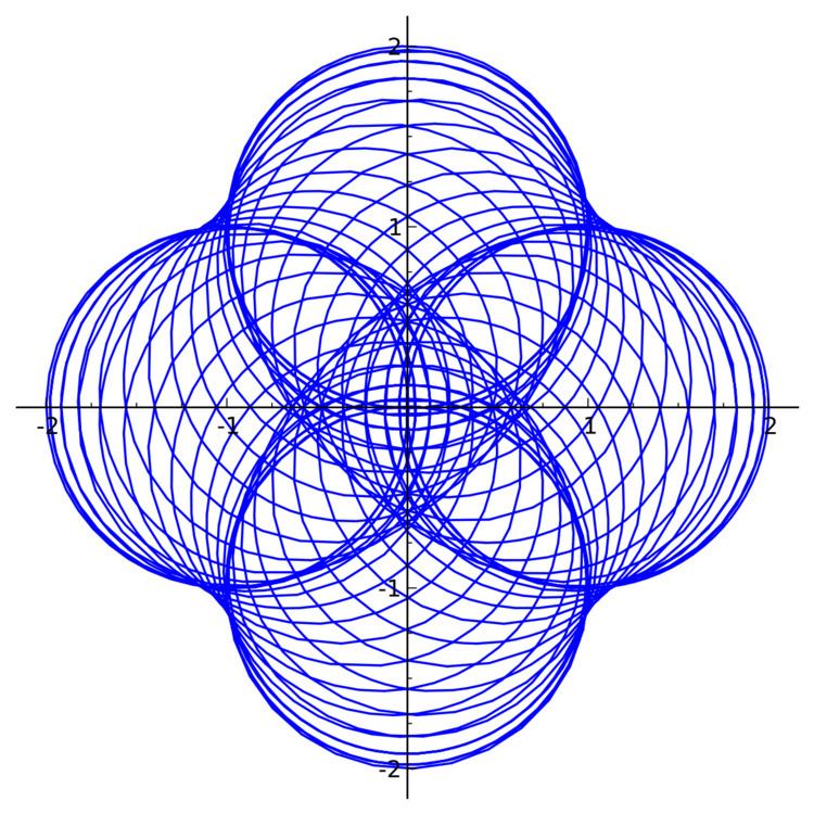
Example 3: n-Curve of the Rhodonea minus the Rhodonea curve

Let us take the Rhodonea Curve

r = cos ( 3 θ )

If ρ denotes the curve,

ρ ( t ) = cos ( 6 π t ) [ cos ( 2 π t ) + i sin ( 2 π t ) ] , 0 t 1

The parametric equations of ρ n ρ are

x = cos ( 6 π n t ) cos ( 2 π n t ) cos ( 6 π t ) cos ( 2 π t ) , y = cos ( 6 π n t ) sin ( 2 π n t ) cos ( 6 π t ) sin ( 2 π t ) , 0 t 1

n-Curving

If γ H , then, as mentioned above, the n-curve γ n  also  H . Therefore, the mapping α γ n 1 α γ n is an inner automorphism of the group G. We extend this map to the whole of C[0, 1], denote it by ϕ γ n , e and call it n-curving with γ. It can be verified that

ϕ γ n , e ( α ) = α + [ α ( 1 ) α ( 0 ) ] ( γ n 1 ) e .  

This new curve has the same initial and end points as α.

Example 1 of n-curving

Let ρ denote the Rhodonea curve r = cos ( 2 θ ) , which is a loop at 1. Its parametric equations are

x = cos ( 4 π t ) cos ( 2 π t ) , y = cos ( 4 π t ) sin ( 2 π t ) , 0 t 1

With the loop ρ we shall n-curve the cosine curve

c ( t ) = 2 π t + i cos ( 2 π t ) , 0 t 1.

The curve ϕ ρ n , e ( c ) has the parametric equations

x = 2 π [ t 1 + cos ( 4 π n t ) cos ( 2 π n t ) ] , y = cos ( 2 π t ) + 2 π cos ( 4 π n t ) sin ( 2 π n t )

See the figure.

It is a curve that starts at the point (0, 1) and ends at (2π, 1).

Example 2 of n-curving

Let χ denote the Cosine Curve

χ ( t ) = 2 π t + i cos ( 2 π t ) , 0 t 1

With another Rhodonea Curve

ρ = cos ( 3 θ )

we shall n-curve the cosine curve.

The rhodonea curve can also be given as

ρ ( t ) = cos ( 6 π t ) [ cos ( 2 π t ) + i sin ( 2 π t ) ] , 0 t 1

The curve ϕ ρ n , e ( χ ) has the parametric equations

x = 2 π t + 2 π [ cos ( 6 π n t ) cos ( 2 π n t ) 1 ] , y = cos ( 2 π t ) + 2 π cos ( 6 π n t ) sin ( 2 π n t ) , 0 t 1

See the figure for n = 15 .

Generalized n-curving

In the FTA C[0, 1] of curves, instead of e we shall take an arbitrary curve β , a loop at 1. This is justified since

L 1 ( β ) = L 2 ( β ) = 1

Then, for a curve γ in C[0, 1],

γ = ( γ ( 0 ) + γ ( 1 ) ) β γ

and

γ 1 = γ γ ( 0 ) γ ( 1 ) .

If α H , the mapping

ϕ α n , β

given by

ϕ α n , β ( γ ) = α n 1 γ α n

is the n-curving. We get the formula

ϕ α n , β ( γ ) = γ + [ γ ( 1 ) γ ( 0 ) ] ( α n β ) .

Thus given any two loops α and β at 1, we get a transformation of curve

γ given by the above formula.

This we shall call generalized n-curving.

Example 1

Let us take α and β as the unit circle ``u.’’ and γ as the cosine curve

γ ( t ) = 4 π t + i cos ( 4 π t ) 0 t 1

Note that γ ( 1 ) γ ( 0 ) = 4 π

For the transformed curve for n = 40 , see the figure.

The transformed curve ϕ u n , u ( γ ) has the parametric equations

Example 2

Denote the curve called Crooked Egg by η whose polar equation is

r = cos 3 θ + sin 3 θ

Its parametric equations are

x = cos ( 2 π t ) ( cos 3 2 π t + sin 3 2 π t ) , y = sin ( 2 π t ) ( cos 3 2 π t + sin 3 2 π t )

Let us take α = η and β = u ,

where u is the unit circle.

The n-curved Archimedean spiral has the parametric equations

x = 2 π t cos ( 2 π t ) + 2 π [ ( cos 3 2 π n t + sin 3 2 π n t ) cos ( 2 π n t ) cos ( 2 π t ) ] , y = 2 π t sin ( 2 π t ) + 2 π [ ( cos 3 2 π n t ) + sin 3 2 π n t ) sin ( 2 π n t ) sin ( 2 π t ) ]

See the figures, the Crooked Egg and the transformed Spiral for n = 20 .

References

N-curve Wikipedia