
 | ||
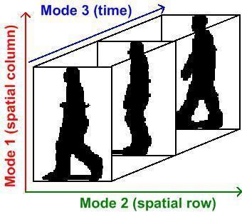
Multilinear subspace learning is an approach to dimensionality reduction. Dimensionality reduction can be performed on data tensor whose observations have been vectorized and organized into a data tensor, or whose observations are matrices that are concatenated into a data tensor. Here are some examples of data tensors whose observations are vectorized or whose observations are matrices concatenated into data tensor images (2D/3D), video sequences (3D/4D), and hyperspectral cubes (3D/4D).
Contents
- Background
- Multilinear Principal Component Analysis
- Multilinear Independent Component Analysis
- Multilinear Linear Descriminant Analysis
- Multilinear canonical correlation analysis
- Typical approach in MSL
- Pros and cons
- Code
- Tensor data sets
- References
The mapping from a high-dimensional vector space to a set of lower dimensional vector spaces is a multilinear projection.
Multilinear subspace learning algorithms are higher-order generalizations of linear subspace learning methods such as principal component analysis (PCA), independent component analysis (ICA), linear discriminant analysis (LDA) and canonical correlation analysis (CCA).
Background
With the advances in data acquisition and storage technology, big data (or massive data sets) are being generated on a daily basis in a wide range of emerging applications. Most of these big data are multidimensional. Moreover, they are usually very-high-dimensional, with a large amount of redundancy, and only occupying a part of the input space. Therefore, dimensionality reduction is frequently employed to map high-dimensional data to a low-dimensional space while retaining as much information as possible.
Linear subspace learning algorithms are traditional dimensionality reduction techniques that represent input data as vectors and solve for an optimal linear mapping to a lower-dimensional space. Unfortunately, they often become inadequate when dealing with massive multidimensional data. They result in very-high-dimensional vectors, lead to the estimation of a large number of parameters.
Multilinear Subspace Learning employ different types of data tensor analysis tools for dimensionality reduction. Multilinear Subspace learning can be applied to observations whose measurements were vectorized and organized into a data tensor, or whose measurements are treated as a matrix and concatenated into a tensor.
Multilinear Principal Component Analysis
Historically, Multilinear Principal Component Analysis has been referred to as "M-mode PCA", a terminology which was coined by Peter Kroonenberg. In 2005, Vasilescu and Terzopoulos introduced the Multilinear PCA terminology as a way to better differentiate between linear tensor decompositions and multilinear tensor decomposition, as well as, to better differentiate between analysis approaches that computed 2nd order statistics associated with each data tensor mode(axis)s, and subsequent work on Multilinear Independent Component Analysis that computed higher order statistics associated with each tensor mode/axis. MPCA is an extension of PCA.
Multilinear Independent Component Analysis
Multilinear Independent Component Analysis is an extension of ICA.
Multilinear Linear Descriminant Analysis
Multilinear canonical correlation analysis
Typical approach in MSL
There are N sets of parameters to be solved, one in each mode. The solution to one set often depends on the other sets (except when N=1, the linear case). Therefore, the suboptimal iterative procedure in is followed.
- Initialization of the projections in each mode
- For each mode, fixing the projection in all the other mode, and solve for the projection in the current mode.
- Do the mode-wise optimization for a few iterations or until convergence.
This is originated from the alternating least square method for multi-way data analysis.
Pros and cons
The advantages of MSL are:
The disadvantages of MSL are: