
 | ||
Moving horizon estimation (MHE) is an optimization approach that uses a series of measurements observed over time, containing noise (random variations) and other inaccuracies, and produces estimates of unknown variables or parameters. Unlike deterministic approaches like the Kalman filter, MHE requires an iterative approach that relies on linear programming or nonlinear programming solvers to find a solution.
Contents
MHE reduces to the Kalman filter under certain simplifying conditions. A critical evaluation of the extended Kalman filter and MHE found improved performance of MHE with the only cost of improvement being the increased computational expense. Because of the computational expense, MHE has generally been applied to systems where there are greater computational resources and moderate to slow system dynamics. However, in the literature there are some methods to accelerate this method.
Overview
The application of MHE is generally to estimate measured or unmeasured states of dynamical systems. Initial conditions and parameters within a model are adjusted by MHE to align measured and predicted values. MHE is based on a finite horizon optimization of a process model and measurements. At time t the current process state is sampled and a minimizing strategy is computed (via a numerical minimization algorithm) for a relatively short time horizon in the past:
Principles of MHE
Moving horizon estimation (MHE) is a multivariable estimation algorithm that uses:
to calculate the optimum states and parameters.
The optimization estimation function is given by:
without violating state or parameter constraints (low/high limits)
With:
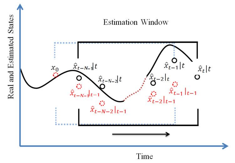
Moving horizon estimation uses a sliding time window. At each sampling time the window moves one step forward. It estimates the states in the window by analyzing the measured output sequence and uses the last estimated state out of the window, as the prior knowledge.