
 | ||
Several techniques can be used to move signals in the time-frequency distribution. Similar to computer graphic techniques, signals can be subjected to horizontal shifting, vertical shifting, dilation (scaling), shearing, and rotation. These techniques can help to save the bandwidth with proper motions apply on the signals. Moreover, filters with proper motion transformation can save the hardware cost without additional filters.
Contents
- Shifting
- Horizontal shifting
- Vertical shifting
- Dilation
- time stretching
- Shearing
- On Vertical axis only frequency
- On Horizontal axis only time
- Rotation
- Clockwise rotation by 90 degrees
- Counterclockwise rotation by 90 degrees
- Rotation by 180 degrees
- Example
- Applications
- References
The following examples assume time in the horizontal axis versus frequency in the vertical axis. As a coincident, the following transformations happen to have the motion properties in the time-frequency distribution.
Shifting
Shifting on time axis is like horizontal shifting in time-frequency distribution. On another hand, shifting on the frequency axis would be vertical shifting in time-frequency distribution.
Horizontal shifting
If t0 is greater than 0, we would be shifting the signal to the right on time axis. (negative would be left)
STFT, Gabor:
WDF:
Vertical shifting
If f0 is greater than 0, we would be shifting the signal to the upward on frequency axis. (negative would be downward)
STFT, Gabor:
WDF:
This results in an amplitude modulation signal. This sort of shift is also used in a frequency extender. This sort of shift is also used in most bat detectors.
Such an effect is typically implemented using heterodyning
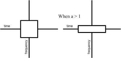
Dilation
Dilation is like doing scaling on one of the axis and area is the same after the process. When a > 1, it's expanding on time axis, and narrowing on frequency axis ;vice versa when a < 1.
STFT, Gabor:
WDF:
When this kind of dilation is applied to audio, it causes a chipmunk effect.
time stretching
Time stretching is doing scaling only on the time axis, leaving frequencies the same. When a < 1 (the most common case), it's narrowing on the time axis, reducing the area.
STFT, Gabor:
WDF:
Shearing
Shearing by definition is moving the side of the signal on one direction. Vertical and Horizontal shearing is introduced here.
On Vertical axis only (frequency)
It's shearing on frequency axis, since this only changes the phase.
STFT, Gabor:
WDF:
On Horizontal axis only (time)
It's shearing on time axis, since this only changes the time.
STFT, Gabor:
WDF:
Rotation
Many transforms has the property of rotations, like Gabor-Wigner, Ambiguity function (counterclockwise), modified Wigner, Cohen's class distribution.
STFT, Gabor, and WDF is introduced in here.
Clockwise rotation by 90 degrees
By switching the time and negative frequency to frequency and time would act like rotating 90 degrees clockwise.
STFT:
Gabor:
WDF:
Counterclockwise rotation by 90 degrees
By switching the negative time and frequency to frequency and time would act like rotating 90 degrees counterclockwise.
If
Rotation by 180 degrees
Changing the sign of both time and frequency would be like flipping twice on both axis, and it ends up like doing 180 degrees rotation.
If
Example
If we want the left image to become the right image, we can use the techniques from above to achieve the requirement.
There are several ways to solve this problem, this is one of the possible solutions.
First, we apply clockwise rotation of 90 degree by using one of the transform.
STFT:
Gabor:
WDF:
Second, we set a = 1/3, and perform a horizontal shearing on t-axis.
STFT, Gabor:
WDF:
Third, we shift the signal 2 to the right on t-axis by setting t0 = 2
STFT, Gabor:
WDF:
Finally, we shift the signal 1 to the left on f-axis by setting f0 = -1
STFT, Gabor:
WDF:
Applications
As mentioned in the introduction, the above techniques can be used to save the bandwidth or the filter cost.
Assume the signal look like this.
.
The dashed box is the filter, and the area of the dashed box would be the bandwidth required.
After some operations like the above example, the signal turn into the position like this.
As a result, the bandwidth was saved, since the area became smaller. Moreover, only a lowpass filter is required to recover the signal, instead of a bandpass filter.