Montgomery curve

Definition

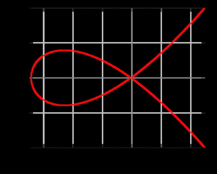
A Montgomery curve over a field K is defined by the equation

for certain A, B ∈ K and with B(A² − 4) ≠ 0.

Generally this curve is considered over a finite field K (for example, over a finite field of q elements, K = F_q) with characteristic different from 2 and with A ∈ K ∖ {−2, 2}, B ∈ K ∖ {0}, but they are also considered over the rationals with the same restrictions for A and B.

Montgomery arithmetic

It is possible to do some "operations" between the points of an elliptic curve: "adding" two points P , Q consists of finding a third one R such that R = P + Q ; "doubling" a point consists of computing [ 2 ] P = P + P (For more information about operations see The group law) and below.

A point P = ( x , y ) on the elliptic curve in the Montgomery form B y 2 = x 3 + A x 2 + x can be represented in Montgomery coordinates P = ( X : Z ) , where P = ( X : Z ) are projective coordinates and x = X / Z for Z ≠ 0 .

Notice that this kind of representation for a point loses information: indeed, in this case, there is no distinction between the affine points ( x , y ) and ( x , − y ) because they are both given by the point ( X : Z ) . However, with this representation it is possible to obtain multiples of points, that is, given P = ( X : Z ) , to compute [ n ] P = ( X n : Z n ) .

Now, considering the two points P n = [ n ] P = ( X n : Z n ) and P m = [ m ] P = ( X m : Z m ) : their sum is given by the point P m + n = P m + P n = ( X m + n : Z m + n ) whose coordinates are:

X m + n = Z m − n ( ( X m − Z m ) ( X n + Z n ) + ( X m + Z m ) ( X n − Z n ) ) 2

Z m + n = X m − n ( ( X m − Z m ) ( X n + Z n ) − ( X m + Z m ) ( X n − Z n ) ) 2

If m = n , then the operation becomes a "doubling"; the coordinates of [ 2 ] P n = P n + P n = P 2 n = ( X 2 n : Z 2 n ) are given by the following equations:

4 X n Z n = ( X n + Z n ) 2 − ( X n − Z n ) 2

X 2 n = ( X n + Z n ) 2 ( X n − Z n ) 2

Z 2 n = ( 4 X n Z n ) ( ( X n − Z n ) 2 + ( ( A + 2 ) / 4 ) ( 4 X n Z n ) )

The first operation considered above (addition) has a time-cost of 3M+2S, where M denotes the multiplication between two general elements of the field on which the elliptic curve is defined, while S denotes squaring of a general element of the field.

The second operation (doubling) has a time-cost of 2M+2S+1D, where D denotes the multiplication of a general element by a constant; notice that the constant is ( A + 2 ) / 4 , so A can be chosen in order to have a small D.

Algorithm and example

The following algorithm represents a doubling of a point P 1 = ( X 1 : Z 1 ) on an elliptic curve in the Montgomery form.

It is assumed that Z 1 = 1 . The cost of this implementation is 1M + 2S + 1*A + 3add + 1*4. Here M denotes the multiplications required, S indicates the squarings, and a refers to the multiplication by A.

Example

Let P 1 = ( 2 , 3 ) be a point on the curve 2 y 2 = x 3 − x 2 + x . In coordinates ( X 1 : Z 1 ) , with x 1 = X 1 / Z 1 , P 1 = ( 2 : 1 ) .

Then:

The result is the point P 3 = ( X 3 : Z 3 ) = ( 9 : 24 ) such that P 3 = 2 P 1 .

Addition

Given two points P 1 = ( x 1 , y 1 ) , P 2 = ( x 2 , y 2 ) on the Montgomery curve M A , B in affine coordinates, the point P 3 = P 1 + P 2 represents, geometrically the third point of intersection between M A , B and the line passing through P 1 and P 2 . It is possible to find the coordinates ( x 3 , y 3 ) of P 3 , in the following way:

1) consider a generic line   y = l x + m in the affine plane and let it pass through P 1 and P 2 (impose the condition), in this way, one obtains l = y 2 − y 1 x 2 − x 1 and m = y 1 − ( y 2 − y 1 x 2 − x 1 ) x 1 ;

2) intersect the line with the curve M A , B , substituting the   y variable in the curve equation with   y = l x + m ; the following equation of third degree is obtained:

x 3 + ( A − B l 2 ) x 2 + ( 1 − 2 B l m ) x − B m 2 = 0 .

As it has been observed before, this equation has three solutions that correspond to the   x coordinates of P 1 , P 2 and P 3 . In particular this equation can be re-written as:

( x − x 1 ) ( x − x 2 ) ( x − x 3 ) = 0

3) Comparing the coefficients of the two identical equations given above, in particular the coefficients of the terms of second degree, one gets:

− x 1 − x 2 − x 3 = A − B l 2 .

So, x 3 can be written in terms of x 1 , y 1 , x 2 , y 2 , as:

x 3 = B ( y 2 − y 1 x 2 − x 1 ) 2 − A − x 1 − x 2 .

4) To find the   y coordinate of the point P 3 it is sufficient to substitute the value x 3 in the line   y = l x + m . Notice that this will not give the point P 3 directly. Indeed, with this method one find the coordinates of the point   R such that R + P 1 + P 2 = P ∞ , but if one needs the resulting point of the sum between P 1 and P 2 , then it is necessary to observe that: R + P 1 + P 2 = P ∞ if and only if − R = P 1 + P 2 . So, given the point   R , it is necessary to find   − R , but this can be done easily by changing the sign to the   y coordinate of   R . In other words, it will be necessary to change the sign of the   y coordinate obtained by substituting the value x 3 in the equation of the line.

Resuming, the coordinates of the point P 3 = ( x 3 , y 3 ) , P 3 = P 1 + P 2 are:

x 3 = B ( y 2 − y 1 ) 2 ( x 2 − x 1 ) 2 − A − x 1 − x 2 = B ( x 2 y 1 − x 1 y 2 ) 2 x 1 x 2 ( x 2 − x 1 ) 2

y 3 = ( 2 x 1 + x 2 + A ) ( y 2 − y 1 ) x 2 − x 1 − B ( y 2 − y 1 ) 3 ( x 2 − x 1 ) 3 − y 1

Doubling

Given a point P 1 on the Montgomery curve M A , B , the point [ 2 ] P 1 represents geometrically the third point of intersection between the curve and the line tangent to P 1 ; so, to find the coordinates of the point P 3 = 2 P 1 it is sufficient to follow the same method given in the addition formula; however, in this case, the line y=lx+m has to be tangent to the curve at P 1 , so, if M A , B : f ( x , y ) = 0 with

f ( x , y ) = x 3 + A x 2 + x − B y 2 ,

then the value of l, which represents the slope of the line, is given by:

l = − ∂ f ∂ x / ∂ f ∂ y

by the implicit function theorem.

So l = 3 x 1 2 + 2 A x 1 + 1 2 B y 1 and the coordinates of the point P 3 , P 3 = 2 P 1 are:

x 3 = B l 2 − A − x 1 − x 1 = B ( 3 x 1 2 + 2 A x 1 + 1 ) 2 ( 2 B y 1 ) 2 − A − x 1 − x 1 = ( x 1 2 − 1 ) 2 4 B y 1 2 = ( x 1 2 − 1 ) 2 4 x 1 ( x 1 2 + A x 1 + 1 )

y 3 = ( 2 x 1 + x 1 + A ) l − B l 3 − y 1 = ( 2 x 1 + x 1 + A ) ( 3 x 1 2 + 2 A x 1 + 1 ) 2 B y 1 − B ( 3 x 1 2 + 2 A x 1 + 1 ) 3 ( 2 B y 1 ) 3 − y 1 .

Equivalence with twisted Edwards curves

Let K be a field with characteristic different from 2.

Let M A , B be an elliptic curve in the Montgomery form:

M A , B : B v 2 = u 3 + A u 2 + u

with A ∈ K ∖ { − 2 , 2 } , B ∈ K ∖ { 0 }

and let E a , d be an elliptic curve in the twisted Edwards form:

with a , d ∈ K ∖ { 0 } , a ≠ d .

The following theorem shows the birational equivalence between Montgomery curves and twisted Edwards curves:

Theorem (i) Every twisted Edwards curve is birationally equivalent to a Montgomery curve over K . In particular, the twisted Edwards curve E a , d is birationally equivalent to the Montgomery curve M A , B where A = 2 ( a + d ) a − d , and B = 4 a − d .

The map:

is a birational equivalence from E a , d to M A , B , with inverse:

Notice that this equivalence between the two curves is not valid everywhere: indeed the map ψ is not defined at the points v = 0 or u + 1 = 0 of the M A , B .

Equivalence with Weierstrass curves

Any elliptic curve can be written in Weierstrass form.

So, the elliptic curve in the Montgomery form

M A , B : B y 2 = x 3 + A x 2 + x ,

can be transformed in the following way: divide each term of the equation for M A , B by B 3 , and substitute the variables x and y, with u = x B and v = y B respectively, to get the equation

v 2 = u 3 + A B u 2 + 1 B 2 u .

To obtain a short Weierstrass form from here, it is sufficient to replace u with the variable t − A 3 B :

v 2 = ( t − A 3 B ) 3 + A B ( t − A 3 B ) 2 + 1 B 2 ( t − A 3 B ) ;

finally, this gives the equation:

v 2 = t 3 + ( 3 − A 2 3 B 2 ) t + ( 2 A 3 − 9 A 27 B 3 ) .

Hence the mapping is given as