Mollifier - Alchetron, The Free Social Encyclopedia

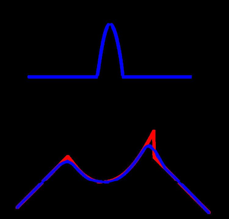
In mathematics, mollifiers (also known as approximations to the identity) are smooth functions with special properties, used for example in distribution theory to create sequences of smooth functions approximating nonsmooth (generalized) functions, via convolution. Intuitively, given a function which is rather irregular, by convolving it with a mollifier the function gets "mollified", that is, its sharp features are smoothed, while still remaining close to the original nonsmooth (generalized) function. They are also known as Friedrichs mollifiers after Kurt Otto Friedrichs, who introduced them.

Modern (distribution based) definition

Definition 1. If φ is a smooth function on ℝⁿ, n ≥ 1, satisfying the following three requirements

(1) it is compactly supported (2) ∫ R n φ ( x ) d x = 1 (3) lim ϵ → 0 φ ϵ ( x ) = lim ϵ → 0 ϵ − n φ ( x / ϵ ) = δ ( x )

where δ ( x ) is the Dirac delta function and the limit must be understood in the space of Schwartz distributions, then φ is a mollifier. The function φ could also satisfy further conditions: for example, if it satisfies

(4) φ ( x ) ≥ 0 for all x ∈ ℝⁿ, then it is called a positive mollifier (5) φ ( x ) = μ ( | x | ) for some infinitely differentiable function μ : ℝ⁺ → ℝ, then it is called a symmetric mollifier

Notes on Friedrichs' definition

Note 1. When the theory of distributions was still not widely known nor used, property (3) above was formulated by saying that the convolution of the function φ ϵ with a given function belonging to a proper Hilbert or Banach space converges as ε → 0 to this last one: this is exactly what Friedrichs did. This also clarifies why mollifiers are related to approximate identities.

Note 2. As briefly pointed out in the "Historical notes" section of this entry, originally, the term "mollifier" identified the following convolution operator:

Φ ϵ ( f ) ( x ) = ∫ R n φ ϵ ( x − y ) f ( y ) d y

where φ ϵ ( x ) = ϵ − n φ ( x / ϵ ) and φ is a smooth function satisfying the first three conditions stated above and one or more supplementary conditions as positivity and symmetry.

Concrete example

Consider the function φ ( x ) of a variable in ℝⁿ defined by

φ ( x ) = { e − 1 / ( 1 − | x | 2 ) / I n if | x | < 1 0 if | x | ≥ 1

where the numerical constant I n ensures normalization. It is easily seen that this function is infinitely differentiable, non analytic with vanishing derivative for |x| = 1. φ can be therefore used as mollifier as described above: it is also easy to see that φ ( x ) defines a positive and symmetric mollifier.

Properties

All properties of a mollifier are related to its behaviour under the operation of convolution: we list the following ones, whose proofs can be found in every text on distribution theory.

Smoothing property

For any distribution T , the following family of convolutions indexed by the real number ϵ

T ϵ = T ∗ φ ϵ

where ∗ denotes convolution, is a family of smooth functions.

Approximation of identity

For any distribution T , the following family of convolutions indexed by the real number ϵ converges to T

lim ϵ → 0 T ϵ = lim ϵ → 0 T ∗ φ ϵ = T ∈ D ′ ( R n )

Support of convolution

For any distribution T ,

s u p p T ϵ = s u p p ( T ∗ φ ϵ ) ⊂ s u p p T + s u p p φ ϵ

where s u p p indicates the support in the sense of distributions, and + indicates their Minkowski addition.

Applications

The basic applications of mollifiers is to prove properties valid for smooth functions also in nonsmooth situations:

Product of distributions

In some theories of generalized functions, mollifiers are used to define the multiplication of distributions: precisely, given two distributions S and T , the limit of the product of a smooth function and a distribution

lim ϵ → 0 S ϵ ⋅ T = lim ϵ → 0 S ⋅ T ϵ = d e f S ⋅ T

defines (if it exists) their product in various theories of generalized functions.

"Weak=Strong" theorems

Very informally, mollifiers are used to prove the identity of two different kind of extension of differential operators: the strong extension and the weak extension. The paper (Friedrichs 1944) illustrates this concept quite well: however the high number of technical details needed to show what this really means prevent them from being formally detailed in this short description.

Smooth cutoff functions

By convolution of the characteristic function of the unit ball B 1 = { x : | x | < 1 } with the smooth function φ 1 / 2 (defined as in (3) with ϵ = 1 / 2 ), one obtains the function

χ B 1 , 1 / 2 ( x ) = χ B 1 ∗ φ 1 / 2 ( x ) = ∫ R n χ B 1 ( x − y ) φ 1 / 2 ( y ) d y = ∫ B 1 / 2 χ B 1 ( x − y ) φ 1 / 2 ( y ) d y ( ∵ s u p p ( φ 1 / 2 ) = B 1 / 2 )

which is a smooth function equal to 1 on B 1 / 2 = { x : | x | < 1 / 2 } , with support contained in B 3 / 2 = { x : | x | < 3 / 2 } . This can be seen easily by observing that if | x | ≤ 1 / 2 and | y | ≤ 1 / 2 then | x − y | ≤ 1 . Hence for | x | ≤ 1 / 2 ,

∫ B 1 / 2 χ B 1 ( x − y ) φ 1 / 2 ( y ) d y = ∫ B 1 / 2 φ 1 / 2 ( y ) d y = 1 .

It is easy to see how this construction can be generalized to obtain a smooth function identical to one on a neighbourhood of a given compact set, and equal to zero in every point whose distance from this set is greater than a given ϵ . Such a function is called a (smooth) cutoff function: those functions are used to eliminate singularities of a given (generalized) function by multiplication. They leave unchanged the value of the (generalized) function they multiply only on a given set, thus modifying its support: also cutoff functions are the basic parts of smooth partitions of unity.

References

Mollifier Wikipedia

(Text) CC BY-SA

Contents