Mindlin–Reissner plate theory - Alchetron, the free social encyclopedia

The Mindlin–Reissner theory of plates is an extension of Kirchhoff–Love plate theory that takes into account shear deformations through-the-thickness of a plate. The theory was proposed in 1951 by Raymond Mindlin. A similar, but not identical, theory had been proposed earlier by Eric Reissner in 1945. Both theories are intended for thick plates in which the normal to the mid-surface remains straight but not necessarily perpendicular to the mid-surface. The Mindlin–Reissner theory is used to calculate the deformations and stresses in a plate whose thickness is of the order of one tenth the planar dimensions while the Kirchhoff-Love theory is applicable to thinner plates.

The form of Mindlin–Reissner plate theory that is most commonly used is actually due to Mindlin and is more properly called Mindlin plate theory. The Reissner theory is slightly different. Both theories include in-plane shear strains and both are extensions of Kirchhoff-Love plate theory incorporating first-order shear effects.

Mindlin's theory assumes that there is a linear variation of displacement across the plate thickness but that the plate thickness does not change during deformation. An additional assumption is that the normal stress through the thickness is ignored; an assumption which is also called the plane stress condition. On the other hand, Reissner's theory assumes that the bending stress is linear while the shear stress is quadratic through the thickness of the plate. This leads to a situation where the displacement through-the-thickness is not necessarily linear and where the plate thickness may change during deformation. Therefore, Reissner's theory does not invoke the plane stress condition.

The Mindlin–Reissner theory is often called the first-order shear deformation theory of plates. Since a first-order shear deformation theory implies a linear displacement variation through the thickness, it is incompatible with Reissner's plate theory.

Mindlin theory

Mindlin's theory was originally derived for isotropic plates using equilibrium considerations. A more general version of the theory based on energy considerations is discussed here.

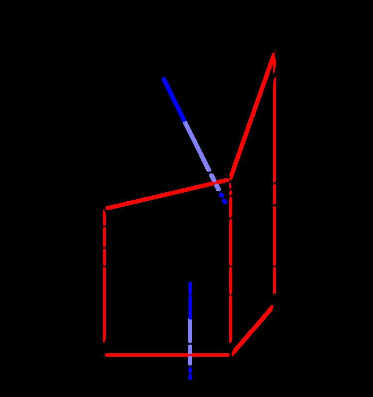
Assumed displacement field

The Mindlin hypothesis implies that the displacements in the plate have the form

u α ( x ) = u α 0 ( x 1 , x 2 ) − x 3 φ α ; α = 1 , 2 u 3 ( x ) = w 0 ( x 1 , x 2 )

where x 1 and x 2 are the Cartesian coordinates on the mid-surface of the undeformed plate and x 3 is the coordinate for the thickness direction, u α 0 , α = 1 , 2 are the in-plane displacements of the mid-surface, w 0 is the displacement of the mid-surface in the x 3 direction, φ 1 and φ 2 designate the angles which the normal to the mid-surface makes with the x 3 axis. Unlike Kirchhoff-Love plate theory where φ α are directly related to w 0 , Mindlin's theory requires that φ 1 ≠ w , 1 0 and φ 2 ≠ w , 2 0 .

Strain-displacement relations

Depending on the amount of rotation of the plate normals two different approximations for the strains can be derived from the basic kinematic assumptions.

For small strains and small rotations the strain–displacement relations for Mindlin–Reissner plates are

ε α β = 1 2 ( u α , β 0 + u β , α 0 ) − x 3 2 ( φ α , β + φ β , α ) ε α 3 = 1 2 ( w , α 0 − φ α ) ε 33 = 0

The shear strain, and hence the shear stress, across the thickness of the plate is not neglected in this theory. However, the shear strain is constant across the thickness of the plate. This cannot be accurate since the shear stress is known to be parabolic even for simple plate geometries. To account for the inaccuracy in the shear strain, a shear correction factor ( κ ) is applied so that the correct amount of internal energy is predicted by the theory. Then

ε α 3 = 1 2 κ ( w , α 0 − φ α )

Equilibrium equations

The equilibrium equations of a Mindlin–Reissner plate for small strains and small rotations have the form

N α β , α = 0 M α β , β − Q α = 0 Q α , α + q = 0

where q is an applied out-of-plane load, the in-plane stress resultants are defined as

N α β := ∫ − h h σ α β d x 3 ,

the moment resultants are defined as

M α β := ∫ − h h x 3 σ α β d x 3 ,

and the shear resultants are defined as

Q α := κ ∫ − h h σ α 3 d x 3 .

Boundary conditions

The boundary conditions are indicated by the boundary terms in the principle of virtual work.

If the only external force is a vertical force on the top surface of the plate, the boundary conditions are

n α N α β o r u β 0 n α M α β o r φ α n α Q α o r w 0

Stress–strain relations

The stress–strain relations for a linear elastic Mindlin–Reissner plate are given by

σ α β = C α β γ θ ε γ θ σ α 3 = C α 3 γ θ ε γ θ σ 33 = C 33 γ θ ε γ θ

Since σ 33 does not appear in the equilibrium equations it is implicitly assumed that it do not have any effect on the momentum balance and is neglected. This assumption is also called the plane stress assumption. The remaining stress–strain relations for an orthotropic material, in matrix form, can be written as

[ σ 11 σ 22 σ 23 σ 31 σ 12 ] = [ C 11 C 12 0 0 0 C 12 C 22 0 0 0 0 0 C 44 0 0 0 0 0 C 55 0 0 0 0 0 C 66 ] [ ε 11 ε 22 ε 23 ε 31 ε 12 ]

Then,

[ N 11 N 22 N 12 ] = ∫ − h h [ C 11 C 12 0 C 12 C 22 0 0 0 C 66 ] [ ε 11 ε 22 ε 12 ] d x 3 = { ∫ − h h [ C 11 C 12 0 C 12 C 22 0 0 0 C 66 ] d x 3 } [ u 1 , 1 0 u 2 , 2 0 1 2 ( u 1 , 2 0 + u 2 , 1 0 ) ]

and

[ M 11 M 22 M 12 ] = ∫ − h h x 3 [ C 11 C 12 0 C 12 C 22 0 0 0 C 66 ] [ ε 11 ε 22 ε 12 ] d x 3 = − { ∫ − h h x 3 2 [ C 11 C 12 0 C 12 C 22 0 0 0 C 66 ] d x 3 } [ φ 1 , 1 φ 2 , 2 1 2 ( φ 1 , 2 + φ 2 , 1 ) ]

For the shear terms

[ Q 1 Q 2 ] = κ ∫ − h h [ C 55 0 0 C 44 ] [ ε 31 ε 32 ] d x 3 = κ 2 { ∫ − h h [ C 55 0 0 C 44 ] d x 3 } [ w , 1 0 − φ 1 w , 2 0 − φ 2 ]

The extensional stiffnesses are the quantities

A α β := ∫ − h h C α β d x 3

The bending stiffnesses are the quantities

D α β := ∫ − h h x 3 2 C α β d x 3 .

Mindlin theory for isotropic plates

For uniformly thick, homogeneous, and isotropic plates, the stress–strain relations in the plane of the plate are

[ σ 11 σ 22 σ 12 ] = E 1 − ν 2 [ 1 ν 0 ν 1 0 0 0 1 − ν ] [ ε 11 ε 22 ε 12 ] .

where E is the Young's modulus, ν is the Poisson's ratio, and ε α β are the in-plane strains. The through-the-thickness shear stresses and strains are related by

σ 31 = 2 G ε 31 and σ 32 = 2 G ε 32

where G = E / ( 2 ( 1 + ν ) ) is the shear modulus.

Constitutive relations

The relations between the stress resultants and the generalized deformations are,

[ N 11 N 22 N 12 ] = 2 E h 1 − ν 2 [ 1 ν 0 ν 1 0 0 0 1 − ν ] [ u 1 , 1 0 u 2 , 2 0 1 2 ( u 1 , 2 0 + u 2 , 1 0 ) ] , [ M 11 M 22 M 12 ] = − 2 E h 3 3 ( 1 − ν 2 ) [ 1 ν 0 ν 1 0 0 0 1 − ν ] [ φ 1 , 1 φ 2 , 2 1 2 ( φ 1 , 2 + φ 2 , 1 ) ] ,

and

[ Q 1 Q 2 ] = κ G 2 h [ w , 1 0 − φ 1 w , 2 0 − φ 2 ] .

The bending rigidity is defined as the quantity

D = 2 E h 3 3 ( 1 − ν 2 ) .

For a plate of thickness h , the bending rigidity has the form

D = E h 3 12 ( 1 − ν 2 ) .

Governing equations

If we ignore the in-plane extension of the plate, the governing equations are

M α β , β − Q α = 0 Q α , α + q = 0 .

In terms of the generalized deformations, these equations can be written as

∇ 2 ( ∂ φ 1 ∂ x 1 + ∂ φ 2 ∂ x 2 ) = − q D ∇ 2 w 0 − ∂ φ 1 ∂ x 1 − ∂ φ 2 ∂ x 2 = − q κ G h ∇ 2 ( ∂ φ 1 ∂ x 2 − ∂ φ 2 ∂ x 1 ) = − 2 κ G h D ( 1 − ν ) ( ∂ φ 1 ∂ x 2 − ∂ φ 2 ∂ x 1 ) .

The boundary conditions along the edges of a rectangular plate are

simply supported w 0 = 0 , M 11 = 0 ( or M 22 = 0 ) , φ 1 = 0 ( or φ 2 = 0 ) clamped w 0 = 0 , φ 1 = 0 , φ 2 = 0 .

Relationship to Reissner theory

The canonical constitutive relations for shear deformation theories of isotropic plates can be expressed as

M 11 = D [ A ( ∂ φ 1 ∂ x 1 + ν ∂ φ 2 ∂ x 2 ) − ( 1 − A ) ( ∂ 2 w 0 ∂ x 1 2 + ν ∂ 2 w 0 ∂ x 2 2 ) ] + q 1 − ν B M 22 = D [ A ( ∂ φ 2 ∂ x 2 + ν ∂ φ 1 ∂ x 1 ) − ( 1 − A ) ( ∂ 2 w 0 ∂ x 2 2 + ν ∂ 2 w 0 ∂ x 1 2 ) ] + q 1 − ν B M 12 = D ( 1 − ν ) 2 [ A ( ∂ φ 1 ∂ x 2 + ∂ φ 2 ∂ x 1 ) − 2 ( 1 − A ) ∂ 2 w 0 ∂ x 1 ∂ x 2 ] Q 1 = A κ G h ( φ 1 + ∂ w 0 ∂ x 1 ) Q 2 = A κ G h ( φ 2 + ∂ w 0 ∂ x 2 ) .

Note that the plate thickness is h (and not 2 h ) in the above equations and D = E h 3 / [ 12 ( 1 − ν 2 ) ] . If we define a Marcus moment,

M = D [ A ( ∂ φ 1 ∂ x 1 + ∂ φ 2 ∂ x 2 ) − ( 1 − A ) ∇ 2 w 0 ] + 2 q 1 − ν 2 B

we can express the shear resultants as

Q 1 = ∂ M ∂ x 1 + D ( 1 − ν ) 2 [ A ∂ ∂ x 2 ( ∂ φ 1 ∂ x 2 − ∂ φ 2 ∂ x 1 ) ] − B 1 + ν ∂ q ∂ x 1 Q 2 = ∂ M ∂ x 2 − D ( 1 − ν ) 2 [ A ∂ ∂ x 1 ( ∂ φ 1 ∂ x 2 − ∂ φ 2 ∂ x 1 ) ] − B 1 + ν ∂ q ∂ x 2 .

These relations and the governing equations of equilibrium, when combined, lead to the following canonical equilibrium equations in terms of the generalized displacements.

∇ 2 ( M − B 1 + ν q ) = − q κ G h ( ∇ 2 w 0 + M D ) = − ( 1 − B c 2 1 + ν ) q ∇ 2 ( ∂ φ 1 ∂ x 2 − ∂ φ 2 ∂ x 1 ) = c 2 ( ∂ φ 1 ∂ x 2 − ∂ φ 2 ∂ x 1 )

where

c 2 = 2 κ G h D ( 1 − ν ) .

In Mindlin's theory, w 0 is the transverse displacement of the mid-surface of the plate and the quantities φ 1 and φ 2 are the rotations of the mid-surface normal about the x 2 and x 1 -axes, respectively. The canonical parameters for this theory are A = 1 and B = 0 . The shear correction factor κ usually has the value 5 / 6 .

On the other hand, in Reissner's theory, w 0 is the weighted average transverse deflection while φ 1 and φ 2 are equivalent rotations which are not identical to those in Mindlin's theory.

Relationship to Kirchhoff-Love theory

If we define the moment sum for Kirchhoff-Love theory as

M K := − D ∇ 2 w K

we can show that

M = M K + B 1 + ν q + D ∇ 2 Φ

where Φ is a biharmonic function such that ∇ 2 ∇ 2 Φ = 0 . We can also show that, if w K is the displacement predicted for a Kirchhoff-Love plate,

w 0 = w K + M K κ G h ( 1 − B c 2 2 ) − Φ + Ψ

where Ψ is a function that satisfies the Laplace equation, ∇ 2 Ψ = 0 . The rotations of the normal are related to the displacements of a Kirchhoff-Love plate by

φ 1 = − ∂ w K ∂ x 1 − 1 κ G h ( 1 − 1 A − B c 2 2 ) Q 1 K + ∂ ∂ x 1 ( D κ G h A ∇ 2 Φ + Φ − Ψ ) + 1 c 2 ∂ Ω ∂ x 2 φ 2 = − ∂ w K ∂ x 2 − 1 κ G h ( 1 − 1 A − B c 2 2 ) Q 2 K + ∂ ∂ x 2 ( D κ G h A ∇ 2 Φ + Φ − Ψ ) + 1 c 2 ∂ Ω ∂ x 1