Mathematics of radio engineering

Spark-gap transmitters and lightning

The existence of electromagnetic waves was first proven by Heinrich Hertz in 1887. After this, there were many public exhibitions of the effect, generally employing very primitive sending and receiving devices. As time went on, experimenters began developing their own devices, and the practice of radio took off. Most often the spark gaps generator where a strong voltage difference between two pieces of metal generates small bolts of lightning.

The problem is the spark is not tuned to a single frequency. Each spike of that intensity in the time domain is a delta function, once passed through a Fourier transform in the frequency domain, covers a large electromagnetic spectrum. Therefore, radio hobbyists at the time were constantly stepping on each other, and there was a lot of interference. Moreover, the efficiency was very low: 99% of the energy went into heat and light, and only one percent went into communications.

AM communications

Experimentation of various ideas lead to transmit only one frequency at a time; or at least reducing the bandwidth so that it would approximate a single frequency. Then, by varying the intensity the signal, usually called the amplitude, AM radio was developed here the message is passed by the modulation. However, it was still somewhat inefficient, because it involved the multiplication of signals, and that generates sidebands, also called sum and difference frequencies. So the information, the sidebands, and anything else to get transmitted. The next step was to send only one sideband, and to block everything else.

The sum and difference frequencies show the value of complex numbers. They exist because the most general expression for a cosine wave is really

where one has both positive and negative frequency components. These occur because a cosine wave is the solution of a linear differential equation, and therefore it obeys the superposition principle: the sum of two solutions is again a solution. This results from the theory of differential equations and these mirror images will not show up on a spectrum analyzer, unless it is designed to display them.

The negative frequencies are sometimes thought of as unimportant, but the sidebands would not exist without them. So when two cosine waves are multiplied, one finds that

The two on the right are the sum and difference, while the two on the left are the negative of those. In the general case ω and ϕ can be any two dimensionless complex numbers, so that the sum and difference may not necessarily lie on the imaginary axis.

It was not long before people began licensing as radio hobbyists, called amateur radio or ham radio. One difficulty was that there were no crystal oscillators then, so they had to design their own frequency generators which used very low frequencies. For instance, if someone were transmitting on 25 kHz, that would be 0.000025 gigahertz. To get an antenna to resonate at that speed, dividing the speed of light by the frequency, a standard half-wavelength antenna would have to be 3.7 miles long which is considered impractical.

Most of the major breakthroughs in radio theory were thus made by hams which remained a strong strong throughout the 70s and 80s. However, with the rise of cell phones and the internet, the number of members is now quite low by comparison.

RLC filters

These are the easiest type of filters to make. The R stands for resistor, the L for inductor, and the C for capacitor. One constructs a loop of copper wire, and connects it to a battery. The elements are placed at different locations in the loop. Mathematically, each loop is a map of the complex plane that simply moves the pole and the zero. The function can signify either impedance or admittance. If one takes the reciprocal, the poles and zeros just switch places.

If one connects a number of these loops together, then one simply gets more poles and zeros moved around. Therefore, one could suppose there is an infinite stack of complex planes; each new current loop takes a pancake off the stack, and moves the poles and zeros around.

One may also start with an infinite number of separate one-loop circuits. One may think of each loop as a potential well, and the current flow as a particle of sorts. Since the loops are not connected, none of the particles know about each other. There is infinite impedance between the current loops. Now if one lowers the impedance between them, then they are affected a little; and if one lowers the impedance even more, then they affected even more. At this point the potential well becomes a complicated surface with many particles bumping into each other.

One may also imagine these starting conditions as a matrix of frequencies. If the matrix is diagonal, then the terms do not affect each other: the sum and product of diagonal matrices is diagonal. But if one introduces off-diagonal elements, then there is an interaction between the terms, and the sum and product of the matrices is more complicated. If one was to assume that the infinite list of frequencies were gradually increasing, and that none were left out, then this would also a way of representing the frequency domain. One could have an oscilloscope that makes graphs with an off-diagonal version of the domain just like this one, and it would still be correct – as long as one did the computations carefully.

One way of adding off-diagonal elements to the admittance matrix x is to multiply it by a non-diagonal matrix a in the following way:

At first this mapping may seems strange, but it has the useful property that the determinant is the same:

This leads to many interesting results. For instance, if n is close to zero, then it represents a small connection between the current loops; the larger it is, the more of a connection there is. This allows a smooth transition from non-interaction to interacting.

Linear vs non-linear filters

All of the above filters are linear. This means that the superposition law holds, or that a generalized version of Ohms law is obeyed. It is often stated as V = IR, where all three are complex matrices. And if there is a bias voltage S, then it can be written as V = S + IR, where S and R are constants. One may interpret this as the first two terms of a taylor series:

where 1 + 3x is simply used as an example of a linear function. Now the series may be continued as

and one has a nonlinear circuit. It is actually true all the time, but the extra terms are usually so small that they are not noticed. The easiest way to generate them is to use a "one-way component" commonly known as a diode. It simply lets the current flow one way and not the other.

Quartz, mechanical and MEMS devices

One of the problems that comes along with these filters is that they don't work very well at higher frequencies. Therefore, one wants to design filters that have a higher quality factor at these frequencies, and this calls for improved technology. The first step in this direction was to notice that crystals behave like a tuning fork, and that they also have very high quality factors. So one feeds the current through a crystal, and it is tuned much better. Another step was the use of mechanical oscillators, which are also very interesting. These are thoroughly described in the article on mechanical filters. Today, the design fabrication process has improved to the point where the dimensions of the objects are surprisingly small, and so the quality factor and the frequencies are much higher. These are known as MEMS devices.

A simpler expression for free waves

Free waves are those that are travelling through the atmosphere, or through empty space; they are not connected with charged particles or currents. These are the types of waves that are transmitted from an antenna, or from a computer. In this case, it is possible to achieve a simplification of the theory. In the absence of charges and currents, Maxwell's equations become

Here one has introduced a complex-valued field E+iB. In this way of thinking, one finds that there is a new symmetry given by

This is a simplification of the theory. The fields are simply rotating, and the frequency is much easier to see. If one were able to plot graphs in three dimensions, one could even use these as a basis for the frequency domain. This is because only the real portion of the waves appear in reality.

Maxwell's equations with quaternions

The algebra of quaternions was discovered by W. R. Hamilton in 1843, and promulgated in his treatise Lectures on Quaternions (1853). Hamilton introduced both real quaternions and complex quaternions, called biquaternions. The algebra was exploited by Peter Guthrie Tait and his school in Scotland, including James Clerk Maxwell, who composed his Maxwell's equations using the facility of vector algebra that quaternion algebra introduced. In the early days there was no set theory or modern algebra to describe the symmetry that Maxwell grasped. Much later, in the evolution of general linear algebra, Hendrik Lorentz expressed the symmetry with the Lorentz transformations.

This idea involves quaternions with complex coefficients, called biquaternions. One defines a four-vector as follows:

where a, b, c and d are real numbers. Then the length of q is

which is nice because it is the Minkowski metric. The Lorentz transform of a biquaternion q has a surprisingly simple form:

The first is a rotation by an angle θ around a three-vector n; the second is a boost by a hyperbolic angle θ in the direction of n. The vector n can be thought of as an element of SU(2), because it has length one, and can point in any of three directions. The star means complex conjugation of the first term. Very similar formulas can be found in the article on quaternions and spatial rotations, which covers this from a purely mathematical viewpoint but does not cover electromagnetism.

Now that invariance under Lorentz transformations has been established, all that is left to do is write the equations in biquaternionic form, and one finds that they reduce to a single equation:

where

The D D ¯ term is interesting. Since each factor D is four-dimensional, the product should be 16-dimensional. Yet the terms intricately cancel, and there are only four left. This is the D'alambert operator, viz

This is really an example of Noether's theorem, which says if there is a symmetry in a certain theory, then there will also be a conservation law in that theory. In this case, the symmetry is the Lorentz group, and what is conserved is Maxwell's equations. The E and B fields become different, but the equations they form do not.

Electromagnetism has been studied from a vast array of viewpoints. The goal is to understand the deeper reasons for it. The most successful generalization is the electroweak theory. More speculative ideas are the SU(5) and SO(10) theories. Some theories are unusually speculative. For instance, if one applies the Cayley–Dickson construction to the quaternions three times over, one arrives at the 32-dimensional "trigintaduonions", in which "it is believed that electromagnetic-gravitational field, strong-weak field, hyper-strong field and hyper-weak field are unified, equal and interconnected." The next section provides a generalization based on the possible existence of both electric and magnetic charge.

A symmetric version of the equations

One notices that electric charge has radial "lines of force" emanating from it. In addition, magnetic poles have concentric "circles of force" radiating from them. One could make a two-dimensional version of this by means of the complex plane. The lines of force are of the form

where k is a constant, and j ranges over all real numbers. For instance, if k is zero, then e^j is a line of force that goes from zero to infinity. On the other hand, the circles of force are of the form

where k is a constant, and ij ranges over all imaginary numbers. For instance, if k is zero, then e^ij is the unit circle. One switches from one to the other by multiplying the exponents by i. Therefore, one might associate electricity with real numbers, and magnetism with imaginary numbers. Since this is only a two-dimensional version of the idea, one would like to rework this into something that is consistent with four-dimensional spacetime, and with the transformations of special relativity.

Many ideas of this kind have led to the concept of dyons. These are hypothetical particles with both electric and magnetic charge; blending them into one allows them to generate one united field. One writes them like this:

where e is the electric charge and g is the magnetic charge. In the previous section, it was shown how Maxwell's equations can be expressed with quaternions. Yet these equations do not include magnetic charge, because it still has not been experimentally observed. The reader may wonder why such ghostly things as magnetic charge should be studied at all. The answer is that it can simplify the equations dramatically, just as complex numbers simplify circuit equations. Also the majority of macroscopic phenomena would be the same if they existed. Finally, they may well exist, but for some unknown reason have not quite been observed yet, despite many searches for them. So in this spirit of adventure, one group of researchers introduce the magnetic counterpart of the quaternionic A and J vectors as follows:

The complete complex quaternionic fields are therefore

The important point is that the two biquaternionic fields match perfectly, because

One may also introduce a magnetic electromagnetic tensor, usually denoted by F^uv, but in this case by iF^uv. Moreover, we have the following symmetries

The researchers go on to derive the complete symmetric equations from these, as well as several other results. It might also be noted that in this way of thinking, there is no divergence, gradient, curl, or vector calculus. Instead, there is only two-by-two matrix multiplication. This is because the complete biquaternion algebra is the same as the algebra of two-by-two complex matrices (in eight dimensions). This makes the subject much easier to work with.

Introduction

While Maxwell's equation were immensely successful in predicting electromagnetic phenomena for most applications, there was still a feeling that they were somehow lacking. Radio theory should be seamlessly blended with the new molecular chemistry and medicine that were developing at that time, and yet it was not. The answer to this dilemma was provided by the theory of path integrals. They simplified and unified many branches of science in a new and unique way.

The idea was that the light waves are replaced by a diffusion process that uses complex numbers. In this way of thinking, there are only interference patterns, similar to how antenna patterns are formed from interference:

Moreover, the field strength was replaced by probability functions. So the waves were still there in the macroscopic realms, but now they were caused by infinitesimal particles.

Antenna patterns

There is a small handheld device known as a field strength meter. One stands in front of the antenna (not recommended when transmitting), and measures the field strength. As one moves around, one gets a feel for the antenna radiation pattern. In theory, one could make a very accurate picture of the antenna pattern with this method, depending on how much time one spends on it. But in the quantum way of thinking, one is really constructing a probability function instead. The same is true for a cell phone. Instead of thinking of the five bars as a field strength, one may interpret them as a probability function; or more accurately, as a probability histogram.

Path integrals as a determinant

Path integrals can be expressed as structures that are related to the determinant of a matrix. For bosons, one computes the permanent; for fermions, the determinant; for anyons, the immanant. They can be thought of as sums of random walks in different arithmetic systems. As the number of random zig-zags approaches infinity, the matrix becomes infinite-dimensional.

It has been mentioned how the superposition principle applies to light and radio waves (that is, bosons). This is why the permanent is used for light and radio waves: complex numbers are added together and they produce interference patterns: these are of the form xy + yx. But a different kind of superposition principle applies to electrons (that is, fermions). Instead of getting stronger when they are the same, they get weaker. And instead of getting weaker when they are different, they get stronger. So in contrast to the case of radio waves, the determinant is used for electrons and other similar particles. Complex "numbers" are added together to produce interference patterns: these are of the form xy − yx. These are difficult to get used to. Anyons are even more unusual, so this article will not go into them in any more detail.

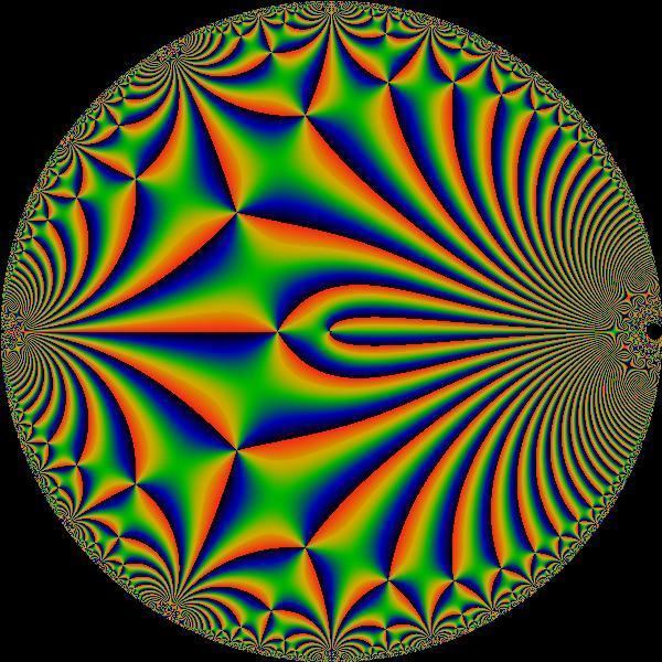
The science of poles and zeros

Complex functions are different from real functions. They are uniquely determined by the poles and zeros. One might imagine a soap bubble that finds a minimal surface of the poles and zeros. If the poles and zeros transform, the soap bubble moves; if they don't, it stays the same.

One of the surprising features is that they can exist at infinity as well. For instance, if there is no distortion at all, the function is zero at zero, and infinity at infinity. This is so obvious that it may be confusing. However it shows an important point: even the plane itself is determined by the poles and zeros. Therefore, they always exist in pairs. Even if there doesn't seem to be an equal number of them, the extra ones are still there.

Another important point is that poles and zeros can be approached from every direction at once. If one moves toward the positive x axis, or the negative x axis, or the positive y axis, or in any direction at all, and keeps going forever, one will arrive at the same point: the point at infinity.

Complex functions also have a dual nature, just as time and frequency response graphs do. In this case, it is the Laplace transform and its inverse that map one to the other. It seems remarkable that the transform can process that much detailed information, and still leave all of the structure the same.

One of the many uses for these functions is as impedance or admittance functions in the analysis of linear systems. This is valuable because every system can be made linear, by looking at smaller and smaller portions of it in the time-frequency domain. Moreover, if one uses several of them to form the basis of a vector space, the system can be n-dimensional.

Useful theorems

There is a long list of useful ideas in complex analysis, going from the reasonably clear to those that are more difficult. Here are several of the best (and easiest) ones. These theorems are stated unusually simply, a bit like crib notes, in order to bring out the meaning.

Reversible computing

If one includes the point at infinity, the complex plane becomes a compact space, and the set of all bijective conformal transformations becomes the Möbius group. Each of these moves the pole and the zero around. Therefore, each is equivalent to a one-loop RLC filter, and the set of one-loop filters is a group as well. However, at least half of these filters are not physically realizable, because the pole is in the right half of the s-plane.

If one starts with an LC filter, adding a positive resistance would cause the oscillations to fade out. One notices that a negative resistance would cause the oscillations to increase. From a mathematical point of view, this is perfectly reasonable. In terms of the Riemann sphere, the former causes the oscillations to converge asymptotically to zero, while the latter causes them to converge asymptotically to infinity, and they are just the mirror-image of each other. The unusual feedback circuits do not emit and dissipate energy, but instead absorb and organize energy. Instead of heating up, a laptop computer would get colder and colder, and could actually serve as a refrigerator.

The central idea here is that of reversibility. One is really allowing time to run backwards, and this is why the computer cools off and creates "reverse entropy". And this is indeed the focus of much current research. Systems of this type are called reversible systems, and they are the heart and soul of quantum computation. Therefore, the concept of conformal transformations is itself transformed, and one arrives at the concept of a unitary transformation of a Hilbert space.

An important point here is that from a topological point of view, all of these filters are identical. Therefore, one may employ big words: every one-loop filter is a diffeomorphism of every other one. This also carries over to higher-order filters: if there are two filters with the same number of poles and zeros, then they are topologically identical, and therefore homeomorphic.

Integral transforms

When astronomers are looking at the sky, they often adjust the telescope in order to refine the results. In the same way, some math problems are easier to solve when they are transformed. This is the idea behind integral transforms: one just rotates the problem to make it simpler.

Linear transformations

As mentioned before, the first two terms of a taylor series are very simple, as follows:

This means that the variable x is multiplied by a factor of three, and the entire thing is moved over by one. If one concentrates solely on the second term, this gives rise to the entire field of group theory. Finite groups are collections of invertible matrices that are applied to a variable. All of the other coefficients can be matrices as well. In this case, the 3 is a one-dimensional matrix in the group of positive real numbers.

The 1 on the other hand, just slides the group over. It is not classified as a linear transformation, but is instead known as an affine transformation. As more terms appear in the power series, things become nonlinear, and the theory becomes more involved. However, in summary, a linear transformation can just be thought of as a matrix.

Fourier, Laplace, Z, Bessel, etc.

All of the integral transforms can be expressed as linear transformations; that is, as matrices. They simply have a different basis. The Fourier transform sends things to one basis, and the Bessel transform to another. One chooses the most convenient basis for studying the problem.

The most important one is the Fourier transform. The entire industry is built on this one idea. Spectrum analyzers and oscilloscopes routinely switch back and forth between different displays by means of the Fourier transform. The next most important is the Laplace transform. It provides useful information on stability and causality of linear systems. Also, one can compute the output just by multiplying the impulse response by the input function. After that there are about twenty or thirty others, and new ones all the time.

One notices that every frequency band of the spectrum can be written as a collection of individual frequencies; that is, complex-valued functions. Therefore, the full spectrum becomes a continuous vector space of functions, sometimes called a topological vector space. The set of subsets forms a lattice (and is also a Boolean algebra in the finite-dimensional case). Another way of saying this is that each subspace each is a direct sum of basis vectors. This allows one to gain more insight into the nature of these integral transforms.

The continuous integral transforms are not really separate from each other. By changing the basis functions infinitesimally, one moves to a different transform. Therefore, each can be rotated into the others.

There are also four-dimensional versions of the transforms, which allow special relativity to play a role. Instead of a basis of functions like

one might replace them with

where t 2 − x 2 − y 2 − z 2 is the minkowski metric and Ω is the four-wave-number. If it were possible to design a spectrum analyzer in four dimensions, then one could generalize the idea of switching back and forth between the time domain and the frequency domain. Instead, one would switch between the spacetime domain and the energy-momentum domain. This carries over to general relativity as well. The most user-friendly version of this theory is called Schwarzschild spacetime. In that case, the Fourier transform is defined also, as long as one stays outside of the photon sphere. The frequency decreases as one climbs up out of the potential well, and therefore one may define a Schwarzschild four-wave-number S. Therefore, the transformer becomes

This generalizes to the next most user-friendly version, which is the Schwarzschild spacetime with a spinning mass and also possibly charged. This is more realistic, because it would seem extremely unlikely that a star would be completely static. But this is beyond the scope of this article.

There are many communications studies which employ the time domain on one axis, and the frequency domain on the other axis. This is two-dimensional. Generalizing to spacetime on one axis and energy-momentum on the other is eight-dimensional. If one is willing to abandon ordinary geometry and go to this symplectic geometry, then one still has a metric space. So one may also define

where t is one-dimensional time, E is one-dimensional energy, x is three-dimensional space, p is three-dimensional momentum, and one is 1 Joule second, in order to make the units come out right.

Duality and lattice theory

In the previous section, one switches back and forth between a basis and its mirror image. Duality theorists take this concept further. They work at rephrasing the totality of science in terms of mirror images. The main idea is expressed in lattice theory. If there exists a set of nested structures, then there exists an algebra as well, with union and intersection playing the role of algebraic operations. Now if one reverses the role of the operations, and also reverses the nesting structure, then one has a dual structure. To reverse the nesting structure means that less-than becomes greater-than, and vice versa; or whatever it was that caused the nesting sequence is reversed; it could be some abstract idea. The entire structure becomes the opposite of what it was.

For example, in the image at the right, one has the lattice of integers that divide the number 60. Now if one considers the lattice of fractions that divide the number 1/60th, then this would be the dual lattice. Even though 1/3rd is more than 1/60th, it still divides it. The next section considers the concept of generalizing this dual idea.

Fractional transformations

A fractional transform is one that rotates around a circle. For instance, the ordinary Fourier transform can be applied at most four times before it starts repeating. In some cases, it will start repeating after only two times. But the fractional transform repeats after a thousand times; it goes around in a circle. Unfortunately it is poorly named, and will be called a rotational transform for the remainder of this article.

These rotational transforms are connected to the theory of Riemann surfaces. For instance, e^ix is a circle, but the inverse function ln(z) is not one-to-one. This can be solved by allowing ln(z) to operate on a helical surface instead. Similarly, the rotational transforms are parameterized by a circle, but the inverse rotational transform is not one-to-one. This can be solved by interpreting the input as a helix as well.

There has been some consideration of applying the helix idea to dual lattices. The prototypical example of a lattice is a Hasse diagram. The leave-it-the-same or reverse-it operations can be though of as the numbers +1 and −1 on the unit circle. This dual structure is now replaced with the circle, which is in turn replaced with a helix. There are various way to approach this problem.

One way is to think of the signal strength on a cell phone, or on the list of wireless connections on a computer. There will four or five bars. They don't appear like this:

but rather like this

This means that they are nested, in some sense. If one is getting 4 bars, then they are still getting 3 bars as well. Therefore, because of the nesting structure, the intersection and union of them forms an algebra. For example,

and

The reverse of this would be the dual lattice.

Another example is provided by the prime numbers: every fraction can be uniquely expressed as a ratio of products of primes. But every fraction can also be expressed uniquely as a ratio of products of these numbers:

For instance

and

A similar idea applies to polynomials. The usual basis for the set of all polynomials is

However, if one constructs the following basis instead

then it has a lattice structure, because each subspace is inside the next one.

One notices that the Fourier transform is not immediately apparent in the previous examples. It can be brought in by thinking in the very same way of a set of frequencies. The usual basis for the frequency domain is

If one constructs this basis instead

then it is nested, and it can be turned into a lattice. The Fourier transform exchanges frequency/time, convolution/multiplication, gcd/lcm, [p mod q]/[q mod p], and so forth. This is the same as turning the lattice upside down, or turning subset into superset. Making this into a rotational helix is analogous to making the circle into a helix for the inverse rotational transforms.

Dual categories

One possible way of unifying these ideas is to employ the fluffy and abstract notions of category theory. There are the ideas of opposite category and dual category. This means the structures are reversed, as well as the operations. One finds that many dual structures become the same in this case. Often there is only one statement, but many different versions of it. This in turn allows one to prove many different theorems at once.

For instance, one might consider the following table:

where the overbar stands for the complement of a set, the dot is pointwise multiplication, and the star is convolution. (GCD and LCM are still defined on the set of fractions, although one may have to work out a few examples to convince oneself that this is true). But as one studies the table, one can see that there is essentially only one statement here, and that the mirror images on the right are the dual statements.

As another example, one might consider the complex fractions. One finds that GCD and LCM are defined for them as well. So one may form the infinite lattice of divisors, just as one would for the real fractions. The added benefit here is that these can be mapped to the Riemann sphere, so that the dual map just reflects about the equator. As one adds more and more irrational roots of unity to the complex fractions, they converge to a finer topology, and one arrives at interesting symmetries in number theory. In this way, the function 1/z plays the role of an abstract Fourier transform, and everything else is the same. In technical jargon, one would say that 1/z is a decategorified Fourier transform.

Thus, many results from ordinary mathematics can be proved in more interesting categories. It might be hoped that the electric and magnetic fields would fit neatly into this particular framework as well, but unfortunately this is not the case. It is now felt by many that "nature does not seem to display exact electromagnetic duality".

Phased antenna arrays

Antenna theory has improved over the years. Instead of just throwing a wire out the window, people are now using antenna arrays. Interference is sometimes thought of as a nuisance, but it can also be a good thing. For instance, if one transmits with a hypothetical omnidirectional antenna, the signal will be transmitted in all directions equally. This might be considered wasteful or non-optimal. If instead, one transmits the very same message with two different antennas, there will be a clearly defined interference pattern, with a stronger signal in some directions, and a weaker signal in others. By using more and more antennas, the radiation pattern can be made very precise. And because the transmit pattern is the same as the reception pattern, it allows them to receive in precise directions as well. In addition, the arrays are able to adjust themselves for better reception. This is where the term adaptive antenna array comes from. It is accomplished with various optimization techniques.

Digital radio

Some of the articles on Wikipedia say that certain things are a little easier with digital radio. This is not correct. The truth is that one achieves spectacularly superior results with digital radio, than one could ever achieve with pure analog circuits alone. This is because the filtering techniques, radiation patterns, gain, impedance matching, and almost everything else can be revised by a programmer quite easily. In many cases, it can be revised by the program itself quite easily. The code may be written in C, or in some low level assembly language. An as example, one may imagine trying to log on to Wikipedia with just analog circuits.

However, it is important to realize that even the best programmer should have some knowledge of analog design, because the two concepts work together. Often there is a group of people who are trained in analog, and a separate group who are trained in programming. The best possible scenario would be if each employee had a working knowledge of both, with a few who were expert in one or the other.

System-on-a-chip

Things have come a long way from the days of spark-gap transmitters. The system on a chip is a set-up for integrating all the components of an electronics system into a single integrated circuit. Researchers have also considered systems that employ multiple processor cores. These provide the ability to easily change the functioning of a powerful system in many useful ways. Also there are many suppliers online. Other related technologies are field-programmable gate arrays that offer "partial reconfigurability", and the network-on-chip technology.

Neural networks and AI

Neural networks are the wave of the future. They start with no knowledge, and learn from experience. Often there is no reason for them to stop learning, which means they can accumulate a vast amount of experience. Radar and antenna systems are much more capable and powerful in this way, and sometimes better at making decisions than a human. There is a large amount of research on neural networks in communications theory today. It is only one type of artificial intelligence. Other techniques have been applied to large arrays of MIMO systems. These include estimation theory and Markov chains. Quantum particle swarm optimization is another approach. Another is the stochastic pooling network. It is said to be "applicable to examples in biological neural coding, nano-electronics, distributed sensor networks, digital beamforming arrays, image processing, [and] multiaccess communication".