
 | ||
Markov decision processes (MDPs) provide a mathematical framework for modeling decision making in situations where outcomes are partly random and partly under the control of a decision maker. MDPs are useful for studying a wide range of optimization problems solved via dynamic programming and reinforcement learning. MDPs were known at least as early as the 1950s (cf. Bellman 1957). A core body of research on Markov decision processes resulted from Ronald A. Howard's book published in 1960, Dynamic Programming and Markov Processes. They are used in a wide area of disciplines, including robotics, automated control, economics, and manufacturing.
Contents
- Definition
- Problem
- Algorithms
- Value iteration
- Policy iteration
- Modified policy iteration
- Prioritized sweeping
- Extensions and generalizations
- Partial observability
- Reinforcement learning
- Learning Automata
- Category theoretic interpretation
- Fuzzy Markov decision processes FMDPs
- Continuous time Markov Decision Process
- Linear programming formulation
- Hamilton Jacobi Bellman equation
- Application
- Alternative notations
- Constrained Markov Decision Processes
- References
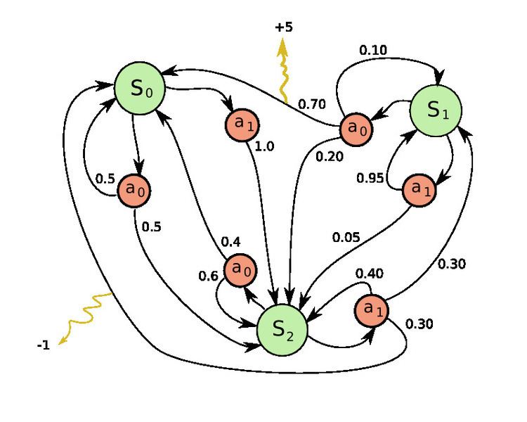
More precisely, a Markov Decision Process is a discrete time stochastic control process. At each time step, the process is in some state
The probability that the process moves into its new state
Markov decision processes are an extension of Markov chains; the difference is the addition of actions (allowing choice) and rewards (giving motivation). Conversely, if only one action exists for each state (e.g. "wait") and all rewards are the same (e.g. "zero"), a Markov decision process reduces to a Markov chain.
Definition
A Markov decision process is a 5-tuple
(Note: The theory of Markov decision processes does not state that
Problem
The core problem of MDPs is to find a "policy" for the decision maker: a function
The goal is to choose a policy
where
Because of the Markov property, the optimal policy for this particular problem can indeed be written as a function of
Algorithms
MDPs can be solved by linear programming or dynamic programming. In what follows we present the latter approach.
Suppose we know the state transition function
The standard family of algorithms to calculate this optimal policy requires storage for two arrays indexed by state: value
The algorithm has the following two kinds of steps, which are repeated in some order for all the states until no further changes take place. They are defined recursively as follows:
Their order depends on the variant of the algorithm; one can also do them for all states at once or state by state, and more often to some states than others. As long as no state is permanently excluded from either of the steps, the algorithm will eventually arrive at the correct solution.
Value iteration
In value iteration (Bellman 1957), which is also called backward induction, the
Substituting the calculation of
where
Policy iteration
In policy iteration (Howard 1960), step one is performed once, and then step two is repeated until it converges. Then step one is again performed once and so on.
Instead of repeating step two to convergence, it may be formulated and solved as a set of linear equations.
This variant has the advantage that there is a definite stopping condition: when the array
Modified policy iteration
In modified policy iteration (van Nunen 1976; Puterman & Shin 1978), step one is performed once, and then step two is repeated several times. Then step one is again performed once and so on.
Prioritized sweeping
In this variant, the steps are preferentially applied to states which are in some way important - whether based on the algorithm (there were large changes in
Extensions and generalizations
A Markov decision process is a stochastic game with only one player.
Partial observability
The solution above assumes that the state
A major advance in this area was provided by Burnetas and Katehakis in "Optimal adaptive policies for Markov decision processes". In this work a class of adaptive policies that possess uniformly maximum convergence rate properties for the total expected finite horizon reward, were constructed under the assumptions of finite state-action spaces and irreducibility of the transition law. These policies prescribe that the choice of actions, at each state and time period, should be based on indices that are inflations of the right-hand side of the estimated average reward optimality equations.
Reinforcement learning
If the probabilities or rewards are unknown, the problem is one of reinforcement learning (Sutton & Barto 1998).
For this purpose it is useful to define a further function, which corresponds to taking the action
While this function is also unknown, experience during learning is based on
Reinforcement learning can solve Markov decision processes without explicit specification of the transition probabilities; the values of the transition probabilities are needed in value and policy iteration. In reinforcement learning, instead of explicit specification of the transition probabilities, the transition probabilities are accessed through a simulator that is typically restarted many times from a uniformly random initial state. Reinforcement learning can also be combined with function approximation to address problems with a very large number of states.
Learning Automata
Another application of MDP process in machine learning theory is called learning automata. This is also one type of reinforcement learning if the environment is in stochastic manner. The first detail learning automata paper is surveyed by Narendra and Thathachar (1974), which were originally described explicitly as finite state automata. Similar to reinforcement learning, learning automata algorithm also has the advantage of solving the problem when probability or rewards are unknown. The difference between learning automata and Q-learning is that they omit the memory of Q-values, but update the action probability directly to find the learning result. Learning automata is a learning scheme with a rigorous proof of convergence.
In learning automata theory, a stochastic automaton to consist of:
The states of such an automaton correspond to the states of a "discrete-state discrete-parameter Markov process". At each time step t=0,1,2,3,..., the automaton reads an input from its environment, updates P(t) to P(t+1) by A, randomly chooses a successor state according to the probabilities P(t+1) and outputs the corresponding action. The automaton's environment, in turn, reads the action and sends the next input to the automaton.
Category theoretic interpretation
Other than the rewards, a Markov decision process
In this way, Markov decision processes could be generalized from monoids (categories with one object) to arbitrary categories. One can call the result
Fuzzy Markov decision processes (FMDPs)
In the MDPs, optimal policy is a policy which maximize the summation of future rewards. Therefore, optimal policy consist several actions which belong to a finite set of actions. In Fuzzy Markov decision processes (FMDPs), first, the value function is computed as regular MDPs i.e. with a finite set of actions; then, the policy is extracted by a fuzzy inference system. In other words, the value function is utilized as an input for the fuzzy inference system, and the policy is the output of the fuzzy inference system.
Continuous-time Markov Decision Process
In discrete-time Markov Decision Processes, decisions are made at discrete time intervals. However, for Continuous-time Markov Decision Processes, decisions can be made at any time the decision maker chooses. In comparison to discrete-time Markov Decision Process, Continuous-time Markov Decision Process can better model the decision making process for a system that has continuous dynamics, i.e., the system dynamics is defined by partial differential equations (PDEs).
Definition
In order to discuss the continuous-time Markov Decision Process, we introduce two sets of notations:
If the state space and action space are finite,
If the state space and action space are continuous,
Problem
Like the Discrete-time Markov Decision Processes, in Continuous-time Markov Decision Process we want to find the optimal policy or control which could give us the optimal expected integrated reward:
Where
Linear programming formulation
If the state space and action space are finite, we could use linear programming to find the optimal policy, which was one of the earliest approaches applied. Here we only consider the ergodic model, which means our continuous-time MDP becomes an ergodic continuous-time Markov Chain under a stationary policy. Under this assumption, although the decision maker can make a decision at any time at the current state, he could not benefit more by taking more than one action. It is better for him to take an action only at the time when system is transitioning from the current state to another state. Under some conditions,(for detail check Corollary 3.14 of Continuous-Time Markov Decision Processes), if our optimal value function
If there exists a function
for all feasible solution
Hamilton-Jacobi-Bellman equation
In continuous-time MDP, if the state space and action space are continuous, the optimal criterion could be found by solving Hamilton-Jacobi-Bellman (HJB) partial differential equation. In order to discuss the HJB equation, we need to reformulate our problem
We could solve the equation to find the optimal control
Application
Continuous-time Markov decision processes have applications in queueing systems, epidemic processes, and population processes.
Alternative notations
The terminology and notation for MDPs are not entirely settled. There are two main streams — one focuses on maximization problems from contexts like economics, using the terms action, reward, value, and calling the discount factor
In addition, transition probability is sometimes written
Constrained Markov Decision Processes
Constrained Markov Decision Processes (CMDPs) are extensions to Markov Decision Process (MDPs). There are three fundamental differences between MDPs and CMDPs.
There are a number of applications for CMDPs. It is recently being used in motion planning scenarios in robotics.