Marginal propensity to save

Calculation

MPS can be calculated as the change in savings divided by the change in income.

M P S = Change in Savings Change in Income

Or mathematically, the marginal propensity to save (MPS) function is expressed as the derivative of the savings (S) function with respect to disposable income (Y).

M P S = d S d Y where, dS=Change in Savings and dY=Change in income.

Now, MPS can be calculated as follows:

Change in savings = (400-200) = 200 Change in income = (1500-1000) = 500

MPS = (Change in savings) / (Change in income)

so, MPS = 200/500 = 0.4

This implies that for each additional one unit of income, the savings increase by 0.4.

There are different implications of this above-mentioned formula.

First it quantifies induced savings.Induced saving is the portion of saving that responds to changes in income. In other words, induced saving can be defined as the household saving that depends on income or production (especially disposable income, national income, or even gross domestic product).

Second, it is a measure of slope of the savings function.

Value

Since MPS is measured as ratio of change in savings to change in income, its value lies between 0 and 1. Also, marginal propensity to save is opposite of marginal propensity to consume.

Mathematically, in a closed economy, MPS + MPC = 1, since an increase in one unit of income will be either consumed or saved.

In the above example, If MPS = 0.4, then MPC = 1 - 0.4 = 0.6.

Generally, it is assumed that value of marginal propensity to save for the richer is more than the marginal propensity to save for the poorer. If income increases for both parties by $1, then the propensity to save for a richer person would be more than that for the poorer person.

Slope of saving line

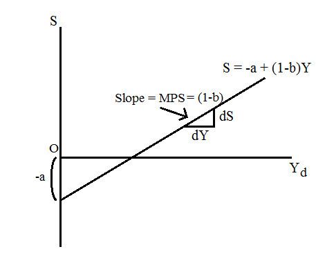
Marginal propensity to save is also used as an alternative term for slope of saving line. The slope of a saving line is given by the equation S = -a + (1-b)Y, where -a refers to autonomous savings and (1-b) refers to marginal propensity to save (here b refers to marginal propensity to consume but as MPC + MPS = 1, so (1-b) refers to MPS).

In this diagram, the savings function is an increasing function of disposable income i.e. savings increase as income increases.

Multiplier effect

An important implication of marginal propensity to save is measurement of the multiplier. A multiplier measures the magnified change in aggregate product i.e. the gross domestic product, resulting from a change in an autonomous variable (for example, government expenditure, investment expenditures, etc.).

The effect of a change in production creates a multiplied impact because it creates income which further creates consumption. However, the resulting consumption is also an expenditure which thus, generates more income, which creates more consumption. This next round of consumption leads to a further change in production, which generates even more income, and which induces even more consumption.

And thus,as it goes on and on, it results in a magnified, multiplied change in aggregate production initially triggered by a change in autonomous variable, but amplified by the creation of more income and increase in consumption.

Mathematical implication

Mathematically, the above effect can be stated as:

In round 1, there is a change in an autonomous variable (say the government invests in a bridge making project for which it approaches a construction company) by an amount $1 (just an assumption for simplification). Now let the marginal propensity to consume for the construction company be 'c'. Thus, the construction company would spend an amount c×$1 i.e. $c.

In round 2, the construction company incurs expenditure ($c) by procuring raw materials, say cement,steel,gravel,mortar,etc. from respective companies and thus, this amount $c becomes income for these companies. Now again the marginal propensity to consume for these companies is same as the construction company at 'c' and thus, their consumption becomes c×$c i.e. $c².

And it goes on and on. We can express this as: Richie

The end result is a magnified, multiplied change in aggregate production initially triggered by the change in investment, but amplified by the change in consumption i.e. the initial investment multiplied by the consumption coefficient (Marginal Propensity to consume).

The MPS enters into the process because it indicates the division of extra income between consumption and saving. It determines how much saving is induced with each change in production and income, and thus how much consumption is induced. If the MPS is smaller, then the multiplier process is also greater as less saving is induced, but more consumption is induced, with each round of activity.

Thus, in this highly simplified model, total magnified change in production due to change in an autonomous variable by $1

= 1 + c + c 2 + ⋯ = 1 1 − c = 1 1 − M P C = 1 M P S

Measuring the multiplier

The effect of a multiplier effect can be measured as:

Simple Multiplier = 1 M P S

If the MPS is smaller, then the multiplier process is also greater as less saving is induced, and more consumption is induced with each round of activity.

For example, if MPS = 0.2, then multiplier effect is 5, and if MPS = 0.4, then the multiplier effect is 2.5. Thus, we can see that a lower propensity to save implies a higher multiplier effect.