Lotka–Volterra equations

History

The Lotka–Volterra predator–prey model was initially proposed by Alfred J. Lotka in the theory of autocatalytic chemical reactions in 1910. This was effectively the logistic equation, which was originally derived by Pierre François Verhulst. In 1920 Lotka extended, via Kolmogorov (see above), the model to "organic systems" using a plant species and a herbivorous animal species as an example and in 1925 he utilised the equations to analyse predator-prey interactions in his book on biomathematics. The same set of equations were published in 1926 by Vito Volterra, a mathematician and physicist who had become interested in mathematical biology. Volterra's enquiry was inspired through his interactions with the marine biologist Umberto D'Ancona who was courting his daughter at the time and later was to become his son-in-law. D'Ancona studied the fish catches in the Adriatic Sea and had noticed that the percentage of predatory fish caught had increased during the years of World War I (1914–18). This puzzled him as the fishing effort had been very much reduced during the war years. Volterra developed his model independently from Lotka and used it to explain d'Ancona's observation.

The model was later extended to include density dependent prey growth and a functional response of the form developed by C.S. Holling; a model that has become known as the Rosenzweig-McArthur model. Both the Lotka–Volterra and Rosenzweig-MacArthur models have been used to explain the dynamics of natural populations of predators and prey, such as the lynx and snowshoe hare data of the Hudson's Bay Company and the moose and wolf populations in Isle Royale National Park.

In the late 1980s an alternative to the Lotka–Volterra predator-prey model (and its common prey dependent generalizations) emerged, the ratio dependent or Arditi–Ginzburg model. The validity of prey or ratio dependent models has been much debated.

In economics

The Lotka–Volterra equations have a long history of use in economic theory; their initial application is commonly credited to Richard Goodwin in 1965 or 1967. In economics, links are between many if not all industries; a proposed way to model the dynamics of various industries has been by introducing trophic functions between various sectors, and ignoring smaller sectors by considering the interactions of only two industrial sectors.

Physical meaning of the equations

The Lotka–Volterra model makes a number of assumptions about the environment and evolution of the predator and prey populations:

1. The prey population finds ample food at all times.
2. The food supply of the predator population depends entirely on the size of the prey population.
3. The rate of change of population is proportional to its size.
4. During the process, the environment does not change in favour of one species and genetic adaptation is inconsequential.
5. Predators have limitless appetite.

As differential equations are used, the solution is deterministic and continuous. This, in turn, implies that the generations of both the predator and prey are continually overlapping.

Prey

When multiplied out, the prey equation becomes

The prey are assumed to have an unlimited food supply, and to reproduce exponentially unless subject to predation; this exponential growth is represented in the equation above by the term αx. The rate of predation upon the prey is assumed to be proportional to the rate at which the predators and the prey meet; this is represented above by βxy. If either x or y is zero then there can be no predation.

With these two terms the equation above can be interpreted as: the change in the prey's numbers is given by its own growth minus the rate at which it is preyed upon.

Predators

The predator equation becomes

In this equation, δ x y represents the growth of the predator population. (Note the similarity to the predation rate; however, a different constant is used as the rate at which the predator population grows is not necessarily equal to the rate at which it consumes the prey). γ y represents the loss rate of the predators due to either natural death or emigration; it leads to an exponential decay in the absence of prey.

Hence the equation expresses the change in the predator population as growth fueled by the food supply, minus natural death.

Solutions to the equations

The equations have periodic solutions and do not have a simple expression in terms of the usual trigonometric functions, although they are quite tractable.

If none of the non-negative parameters α,β,γ,δ vanishes, three can be absorbed into the normalization of variables to leave but merely one behind: Since the first equation is homogeneous in x, and the second one in y, the parameters β/α and δ/γ, are absorbable in the normalizations of y and x, respectively, and γ into the normalization of t, so that only α/γ remains arbitrary. It is the only parameter affecting the nature of the solutions.

A linearization of the equations yields a solution similar to simple harmonic motion with the population of predators trailing that of prey by 90° in the cycle.

A simple example

Suppose there are two species of animals, a baboon (prey) and a cheetah (predator). If the initial conditions are 80 baboons and 40 cheetahs, one can plot the progression of the two species over time. The choice of time interval is arbitrary.

One may also plot solutions parametrically as orbits in "phase-space", without representing time, but with one axis representing the number of prey and the other axis representing the number of predators for all times.

This is to say, eliminating time from the two differential equations above results in only one such,

whose solutions are closed curves. It is amenable to separation of variables: integrating

yields an evident constant quantity V depending on the initial conditions, which is conserved on each curve,

An aside: These graphs illustrate a serious potential problem with this as a biological model: For this specific choice of parameters, in each cycle, the baboon population is reduced to extremely low numbers, yet recovers (while the cheetah population remains sizeable at the lowest baboon density). In real-life situations, however, chance fluctuations of the discrete numbers of individuals, as well as the family structure and life-cycle of baboons, might cause the baboons to actually go extinct, and, by consequence, the cheetahs as well. This modelling problem has been called the "atto-fox problem", an atto-fox being a notional 10⁻¹⁸ of a fox, in the context of rabies modelling in the UK.

Phase-space plot of a further example

A less extreme example covers: α = 2/3, β = 4/3, γ = 1 = δ. Assume x,y quantify thousands, each. Circles represent prey and predator initial conditions from x = y =0.9 to 1.8, in steps of 0.1. The fixed point is at (1,1/2).

Dynamics of the system

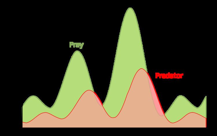
In the model system, the predators thrive when there are plentiful prey but, ultimately, outstrip their food supply and decline. As the predator population is low the prey population will increase again. These dynamics continue in a cycle of growth and decline.

Population equilibrium

Population equilibrium occurs in the model when neither of the population levels is changing, i.e. when both of the derivatives are equal to 0.

When solved for x and y the above system of equations yields

and

Hence, there are two equilibria.

The first solution effectively represents the extinction of both species. If both populations are at 0, then they will continue to be so indefinitely. The second solution represents a fixed point at which both populations sustain their current, non-zero numbers, and, in the simplified model, do so indefinitely. The levels of population at which this equilibrium is achieved depend on the chosen values of the parameters, α, β, γ, and δ.

Stability of the fixed points

The stability of the fixed point at the origin can be determined by performing a linearization using partial derivatives.

The Jacobian matrix of the predator-prey model is

First fixed point (extinction)

When evaluated at the steady state of (0, 0) the Jacobian matrix J becomes

The eigenvalues of this matrix are

In the model α and γ are always greater than zero, and as such the sign of the eigenvalues above will always differ. Hence the fixed point at the origin is a saddle point.

The stability of this fixed point is of significance. If it were stable, non-zero populations might be attracted towards it, and as such the dynamics of the system might lead towards the extinction of both species for many cases of initial population levels. However, as the fixed point at the origin is a saddle point, and hence unstable, it follows that the extinction of both species is difficult in the model. (In fact, this could only occur if the prey were artificially completely eradicated, causing the predators to die of starvation. If the predators were eradicated, the prey population would grow without bound in this simple model): The populations of prey and predator can get infinitesimally close to zero and still recover.

Second fixed point (oscillations)

Evaluating J at the second fixed point leads to

The eigenvalues of this matrix are

As the eigenvalues are both purely imaginary and conjugate to each others, this fixed point is elliptic, so the solutions are periodic, oscillating on a small ellipse around the fixed point, with a period ω = λ 1 λ 2 = α γ   .

As illustrated in the circulating oscillations in the figure above, the level curves are closed orbits surrounding the fixed point: the levels of the predator and prey populations cycle, and oscillate without damping around the fixed point with period ω = α γ .

The value of the constant of motion V, or, equivalently, K=exp(V), : K = y α e − β y x γ e − δ x   , can be found for the closed orbits near the fixed point.

Increasing K moves a closed orbit closer to the fixed point. The largest value of the constant K is obtained by solving the optimization problem

The maximal value of K is thus attained at the stationary (fixed) point ( γ δ , α β ) and amounts to

where e is Euler's Number.