Linear time invariant theory

Overview

The defining properties of any LTI system are linearity and time invariance.

Linearity means that the relationship between the input and the output of the system is a linear map: If input x 1 ( t ) produces response y 1 ( t ) , and input x 2 ( t ) produces response y 2 ( t ) , then the scaled and summed input a 1 x 1 ( t ) + a 2 x 2 ( t ) produces the scaled and summed response a 1 y 1 ( t ) + a 2 y 2 ( t ) where a 1 and a 2 are real scalars. It follows that this can be extended to an arbitrary number of terms, and so for real numbers c 1 , c 2 , … , c k ,

In particular, where c ω and x ω are scalars and inputs that vary over a continuum indexed by ω . Thus if an input function can be represented by a continuum of input functions, combined "linearly", as shown, then the corresponding output function can be represented by the corresponding continuum of output functions, scaled and summed in the same way.

Time invariance means that whether we apply an input to the system now or T seconds from now, the output will be identical except for a time delay of T seconds. That is, if the output due to input x ( t ) is y ( t ) , then the output due to input x ( t − T ) is y ( t − T ) . Hence, the system is time invariant because the output does not depend on the particular time the input is applied.

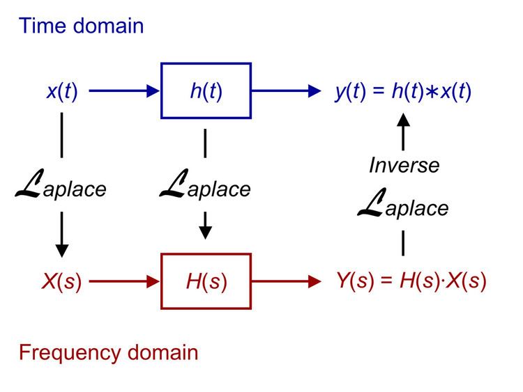
The fundamental result in LTI system theory is that any LTI system can be characterized entirely by a single function called the system's impulse response. The output of the system is simply the convolution of the input to the system with the system's impulse response. This method of analysis is often called the time domain point-of-view. The same result is true of discrete-time linear shift-invariant systems in which signals are discrete-time samples, and convolution is defined on sequences.

Equivalently, any LTI system can be characterized in the frequency domain by the system's transfer function, which is the Laplace transform of the system's impulse response (or Z transform in the case of discrete-time systems). As a result of the properties of these transforms, the output of the system in the frequency domain is the product of the transfer function and the transform of the input. In other words, convolution in the time domain is equivalent to multiplication in the frequency domain.

For all LTI systems, the eigenfunctions, and the basis functions of the transforms, are complex exponentials. This is, if the input to a system is the complex waveform A e s t for some complex amplitude A and complex frequency s , the output will be some complex constant times the input, say B e s t for some new complex amplitude B . The ratio B / A is the transfer function at frequency s .

Since sinusoids are a sum of complex exponentials with complex-conjugate frequencies, if the input to the system is a sinusoid, then the output of the system will also be a sinusoid, perhaps with a different amplitude and a different phase, but always with the same frequency upon reaching steady-state. LTI systems cannot produce frequency components that are not in the input.

LTI system theory is good at describing many important systems. Most LTI systems are considered "easy" to analyze, at least compared to the time-varying and/or nonlinear case. Any system that can be modeled as a linear homogeneous differential equation with constant coefficients is an LTI system. Examples of such systems are electrical circuits made up of resistors, inductors, and capacitors (RLC circuits). Ideal spring–mass–damper systems are also LTI systems, and are mathematically equivalent to RLC circuits.

Most LTI system concepts are similar between the continuous-time and discrete-time (linear shift-invariant) cases. In image processing, the time variable is replaced with two space variables, and the notion of time invariance is replaced by two-dimensional shift invariance. When analyzing filter banks and MIMO systems, it is often useful to consider vectors of signals.

A linear system that is not time-invariant can be solved using other approaches such as the Green function method. The same method must be used when the initial conditions of the problem are not null.

Impulse response and convolution

The behavior of a linear, continuous-time, time-invariant system with input signal x(t) and output signal y(t) is described by the convolution integral:

where h ( t ) is the system's response to an impulse:   x ( τ ) = δ ( τ ) .   y ( t ) is therefore proportional to a weighted average of the input function x ( τ ) .   The weighting function is h ( − τ ) , simply shifted by amount t .   As t changes, the weighting function emphasizes different parts of the input function. When h ( τ ) is zero for all negative τ ,   y ( t ) depends only on values of x prior to time t ,   and the system is said to be causal.

To understand why the convolution produces the output of an LTI system, let the notation { x ( u − τ ) ;   u } represent the function x ( u − τ ) with variable u and constant τ .   And let the shorter notation { x } represent { x ( u ) ;   u } . Then a continuous-time system transforms an input function, { x } , into an output function, { y } . And in general, every value of the output can depend on every value of the input. This concept is represented by:

y ( t )   = def   O t { x } ,

where O t is the transformation operator for time t . In a typical system, y ( t ) depends most heavily on the values of x that occurred near time t .   Unless the transform itself changes with t , the output function is just constant, and the system is uninteresting.

For a linear system, O must satisfy Eq.1 :

And the time-invariance requirement is:

In this notation, we can write the impulse response as   h ( t )   = def   O t { δ ( u ) ;   u } .

Similarly:

Substituting this result into the convolution integral:

x ( t ) ∗ h ( t ) = ∫ − ∞ ∞ x ( τ ) ⋅ h ( t − τ ) d τ = ∫ − ∞ ∞ x ( τ ) ⋅ O t { δ ( u − τ ) ;   u } d τ ,

which has the form of the right side of Eq.2 for the case c τ = x ( τ ) and x τ ( u ) = δ ( u − τ ) .
Eq.2 then allows this continuation:

x ( t ) ∗ h ( t ) = O t { ∫ − ∞ ∞ x ( τ ) ⋅ δ ( u − τ ) d τ ;   u } = O t { x ( u ) ;   u }   = def   y ( t ) .

In summary, the input function, { x } ,   can be represented by a continuum of time-shifted impulse functions, combined "linearly", as shown at Eq.1. The system's linearity property allows the system's response to be represented by the corresponding continuum of impulse responses, combined in the same way.  And the time-invariance property allows that combination to be represented by the convolution integral.

The mathematical operations above have a simple graphical simulation.

Exponentials as eigenfunctions

An eigenfunction is a function for which the output of the operator is a scaled version of the same function. That is,

H f = λ f ,

where f is the eigenfunction and λ is the eigenvalue, a constant.

The exponential functions A e s t , where A , s ∈ C , are eigenfunctions of a linear, time-invariant operator. A simple proof illustrates this concept. Suppose the input is x ( t ) = A e s t . The output of the system with impulse response h ( t ) is then

∫ − ∞ ∞ h ( t − τ ) A e s τ d ⁡ τ

which, by the commutative property of convolution, is equivalent to

∫ − ∞ ∞ h ( τ ) A e s ( t − τ ) d ⁡ τ ⏞ H f = ∫ − ∞ ∞ h ( τ ) A e s t e − s τ d ⁡ τ = A e s t ∫ − ∞ ∞ h ( τ ) e − s τ d ⁡ τ = = A e s t ⏟ Input ⏞ f H ( s ) ⏟ Scalar ⏞ λ ,

where the scalar

H ( s )   = def   ∫ − ∞ ∞ h ( t ) e − s t d ⁡ t

is dependent only on the parameter s.

So the system's response is a scaled version of the input. In particular, for any A , s ∈ C , the system output is the product of the input A e s t and the constant H ( s ) . Hence, A e s t is an eigenfunction of an LTI system, and the corresponding eigenvalue is H ( s ) .

Direct proof

It is also possible to directly derive complex exponentials as eigenfunctions of LTI systems.

Let's set v ( t ) = e i ω t some complex exponential and v a ( t ) = e i ω ( t + a ) a time-shifted version of it.

H [ v a ] ( t ) = e i ω a H [ v ] ( t ) by linearity with respect to the constant e i ω a .

H [ v a ] ( t ) = H [ v ] ( t + a ) by time invariance of H .

So H [ v ] ( t + a ) = e i ω a H [ v ] ( t ) . Setting t = 0 and renaming we get :

H [ v ] ( τ ) = e i ω τ H [ v ] ( 0 )

i.e. that a complex exponential e i ω τ as input will give a complex exponential of same frequency as output.

Fourier and Laplace transforms

The eigenfunction property of exponentials is very useful for both analysis and insight into LTI systems. The Laplace transform

H ( s )   = def   L { h ( t ) }   = def   ∫ − ∞ ∞ h ( t ) e − s t d ⁡ t

is exactly the way to get the eigenvalues from the impulse response. Of particular interest are pure sinusoids (i.e., exponential functions of the form e j ω t where ω ∈ R and j   = def   − 1 ). These are generally called complex exponentials even though the argument is purely imaginary. The Fourier transform H ( j ω ) = F { h ( t ) } gives the eigenvalues for pure complex sinusoids. Both of H ( s ) and H ( j ω ) are called the system function, system response, or transfer function.

The Laplace transform is usually used in the context of one-sided signals, i.e. signals that are zero for all values of t less than some value. Usually, this "start time" is set to zero, for convenience and without loss of generality, with the transform integral being taken from zero to infinity (the transform shown above with lower limit of integration of negative infinity is formally known as the bilateral Laplace transform).

The Fourier transform is used for analyzing systems that process signals that are infinite in extent, such as modulated sinusoids, even though it cannot be directly applied to input and output signals that are not square integrable. The Laplace transform actually works directly for these signals if they are zero before a start time, even if they are not square integrable, for stable systems. The Fourier transform is often applied to spectra of infinite signals via the Wiener–Khinchin theorem even when Fourier transforms of the signals do not exist.

Due to the convolution property of both of these transforms, the convolution that gives the output of the system can be transformed to a multiplication in the transform domain, given signals for which the transforms exist

y ( t ) = ( h ∗ x ) ( t )   = def   ∫ − ∞ ∞ h ( t − τ ) x ( τ ) d ⁡ τ   = def   L − 1 { H ( s ) X ( s ) } .

Not only is it often easier to do the transforms, multiplication, and inverse transform than the original convolution, but one can also gain insight into the behavior of the system from the system response. One can look at the modulus of the system function |H(s)| to see whether the input exp ⁡ ( s t ) is passed (let through) the system or rejected or attenuated by the system (not let through).

Examples

A simple example of an LTI operator is the derivative.

d d ⁡ t ( c 1 x 1 ( t ) + c 2 x 2 ( t ) ) = c 1 x 1 ′ ( t ) + c 2 x 2 ′ ( t )   (i.e., it is linear)

d d ⁡ t x ( t − τ ) = x ′ ( t − τ )   (i.e., it is time invariant)

When the Laplace transform of the derivative is taken, it transforms to a simple multiplication by the Laplace variable s. L { d d ⁡ t x ( t ) } = s X ( s ) That the derivative has such a simple Laplace transform partly explains the utility of the transform.

Another simple LTI operator is an averaging operator

By the linearity of integration, it is linear. Additionally, because it is time invariant. In fact, A can be written as a convolution with the boxcar function Π ( t ) . That is, A { x ( t ) } = ∫ − ∞ ∞ Π ( λ − t 2 a ) x ( λ ) d ⁡ λ , where the boxcar function

Important system properties

Some of the most important properties of a system are causality and stability. Causality is a necessity if the independent variable is time, but not all systems have time as an independent variable. For example, a system that processes still images does not need to be causal. Non-causal systems can be built and can be useful in many circumstances. Even non-real systems can be built and are very useful in many contexts.

Causality

A system is causal if the output depends only on present and past, but not future inputs. A necessary and sufficient condition for causality is

h ( t ) = 0 ∀ t < 0 ,

where h ( t ) is the impulse response. It is not possible in general to determine causality from the Laplace transform, because the inverse transform is not unique. When a region of convergence is specified, then causality can be determined.

Stability

A system is bounded-input, bounded-output stable (BIBO stable) if, for every bounded input, the output is finite. Mathematically, if every input satisfying

  ∥ x ( t ) ∥ ∞ < ∞

leads to an output satisfying

  ∥ y ( t ) ∥ ∞ < ∞

(that is, a finite maximum absolute value of x ( t ) implies a finite maximum absolute value of y ( t ) ), then the system is stable. A necessary and sufficient condition is that h ( t ) , the impulse response, is in L¹ (has a finite L¹ norm):

  ∥ h ( t ) ∥ 1 = ∫ − ∞ ∞ | h ( t ) | d ⁡ t < ∞ .

In the frequency domain, the region of convergence must contain the imaginary axis s = j ω .

As an example, the ideal low-pass filter with impulse response equal to a sinc function is not BIBO stable, because the sinc function does not have a finite L¹ norm. Thus, for some bounded input, the output of the ideal low-pass filter is unbounded. In particular, if the input is zero for t < 0 and equal to a sinusoid at the cut-off frequency for t > 0 , then the output will be unbounded for all times other than the zero crossings.

Discrete-time systems

Almost everything in continuous-time systems has a counterpart in discrete-time systems.

Discrete-time systems from continuous-time systems

In many contexts, a discrete time (DT) system is really part of a larger continuous time (CT) system. For example, a digital recording system takes an analog sound, digitizes it, possibly processes the digital signals, and plays back an analog sound for people to listen to.

Formally, the DT signals studied are almost always uniformly sampled versions of CT signals. If x ( t ) is a CT signal, then an analog to digital converter will transform it to the DT signal:

x [ n ]   = def   x ( n T ) ∀ n ∈ Z ,

where T is the sampling period. It is very important to limit the range of frequencies in the input signal for faithful representation in the DT signal, since then the sampling theorem guarantees that no information about the CT signal is lost. A DT signal can only contain a frequency range of 1 / ( 2 T ) ; other frequencies are aliased to the same range.

Impulse response and convolution

Let { x [ m − k ] ;   m } represent the sequence { x [ m − k ] ;   for all integer values of m } .

And let the shorter notation { x } represent { x [ m ] ;   m } .

A discrete system transforms an input sequence, { x } into an output sequence, { y } . In general, every element of the output can depend on every element of the input. Representing the transformation operator by O , we can write:

y [ n ]   = def   O n { x } .

Note that unless the transform itself changes with n, the output sequence is just constant, and the system is uninteresting. (Thus the subscript, n.) In a typical system, y[n] depends most heavily on the elements of x whose indices are near n.

For the special case of the Kronecker delta function, x [ m ] = δ [ m ] , the output sequence is the impulse response:

h [ n ]   = def   O n { δ [ m ] ;   m } .

For a linear system, O must satisfy:

And the time-invariance requirement is:

In such a system, the impulse response, { h } , characterizes the system completely. I.e., for any input sequence, the output sequence can be calculated in terms of the input and the impulse response. To see how that is done, consider the identity:

x [ m ] ≡ ∑ k = − ∞ ∞ x [ k ] ⋅ δ [ m − k ] ,

which expresses { x } in terms of a sum of weighted delta functions.

Therefore:

y [ n ] = O n { x } = O n { ∑ k = − ∞ ∞ x [ k ] ⋅ δ [ m − k ] ;   m } = ∑ k = − ∞ ∞ x [ k ] ⋅ O n { δ [ m − k ] ;   m } ,

where we have invoked Eq.4 for the case c k = x [ k ] and x k [ m ] = δ [ m − k ] .

And because of Eq.5, we may write:

O n { δ [ m − k ] ;   m }   =   O n − k { δ [ m ] ;   m } = def   h [ n − k ] .

Therefore:

which is the familiar discrete convolution formula. The operator O n can therefore be interpreted as proportional to a weighted average of the function x[k]. The weighting function is h[-k], simply shifted by amount n. As n changes, the weighting function emphasizes different parts of the input function. Equivalently, the system's response to an impulse at n=0 is a "time" reversed copy of the unshifted weighting function. When h[k] is zero for all negative k, the system is said to be causal.

Exponentials as eigenfunctions

An eigenfunction is a function for which the output of the operator is the same function, scaled by some constant. In symbols,

H f = λ f ,

where f is the eigenfunction and λ is the eigenvalue, a constant.

The exponential functions z n = e s T n , where n ∈ Z , are eigenfunctions of a linear, time-invariant operator. T ∈ R is the sampling interval, and z = e s T ,   z , s ∈ C . A simple proof illustrates this concept.

Suppose the input is x [ n ] = z n . The output of the system with impulse response h [ n ] is then

∑ m = − ∞ ∞ h [ n − m ] z m

which is equivalent to the following by the commutative property of convolution

∑ m = − ∞ ∞ h [ m ] z ( n − m ) = z n ∑ m = − ∞ ∞ h [ m ] z − m = z n H ( z )

where

H ( z )   = def   ∑ m = − ∞ ∞ h [ m ] z − m

is dependent only on the parameter z.

So z n is an eigenfunction of an LTI system because the system response is the same as the input times the constant H ( z ) .

Z and discrete-time Fourier transforms

The eigenfunction property of exponentials is very useful for both analysis and insight into LTI systems. The Z transform

H ( z ) = Z { h [ n ] } = ∑ n = − ∞ ∞ h [ n ] z − n

is exactly the way to get the eigenvalues from the impulse response. Of particular interest are pure sinusoids, i.e. exponentials of the form e j ω n , where ω ∈ R . These can also be written as z n with z = e j ω . These are generally called complex exponentials even though the argument is purely imaginary. The Discrete-time Fourier transform (DTFT) H ( e j ω ) = F { h [ n ] } gives the eigenvalues of pure sinusoids. Both of H ( z ) and H ( e j ω ) are called the system function, system response, or transfer function'.

The Z transform is usually used in the context of one-sided signals, i.e. signals that are zero for all values of t less than some value. Usually, this "start time" is set to zero, for convenience and without loss of generality. The Fourier transform is used for analyzing signals that are infinite in extent.

Due to the convolution property of both of these transforms, the convolution that gives the output of the system can be transformed to a multiplication in the transform domain. That is,

y [ n ] = ( h ∗ x ) [ n ] = ∑ m = − ∞ ∞ h [ n − m ] x [ m ] = Z − 1 { H ( z ) X ( z ) } .

Just as with the Laplace transform transfer function in continuous-time system analysis, the Z transform makes it easier to analyze systems and gain insight into their behavior. One can look at the modulus of the system function |H(z)| to see whether the input z n is passed (let through) by the system, or rejected or attenuated by the system (not let through).

Examples

A simple example of an LTI operator is the delay operator D { x [ n ] }   = def   x [ n − 1 ] .

D ( c 1 . x 1 [ n ] + c 2 . x 2 [ n ] ) = c 1 . x 1 [ n − 1 ] + c 2 . x 2 [ n − 1 ] = c 1 . D x 1 [ n ] + c 2 . D x 2 [ n ]   (i.e., it is linear)

D { x [ n − m ] } = x [ n − m − 1 ] = x [ ( n − 1 ) − m ] = D { x } [ n − m ]   (i.e., it is time invariant)

The Z transform of the delay operator is a simple multiplication by z⁻¹. That is, Z { D x [ n ] } = z − 1 X ( z ) .

Another simple LTI operator is the averaging operator

Because of the linearity of sums, and so it is linear. Because, it is also time invariant.

Important system properties

The input-output characteristics of discrete-time LTI system are completely described by its impulse response h [ n ] . Some of the most important properties of a system are causality and stability. Unlike CT systems, non-causal DT systems can be realized. It is trivial to make an acausal FIR system causal by adding delays. It is even possible to make acausal IIR systems. Non-stable systems can be built and can be useful in many circumstances. Even non-real systems can be built and are very useful in many contexts.

Causality

A discrete-time LTI system is causal if the current value of the output depends on only the current value and past values of the input., A necessary and sufficient condition for causality is

h [ n ] = 0   ∀ n < 0 ,

where h [ n ] is the impulse response. It is not possible in general to determine causality from the Z transform, because the inverse transform is not unique. When a region of convergence is specified, then causality can be determined.

Stability

A system is bounded input, bounded output stable (BIBO stable) if, for every bounded input, the output is finite. Mathematically, if

  ∥ x [ n ] ∥ ∞ < ∞

implies that

  ∥ y [ n ] ∥ ∞ < ∞

(that is, if bounded input implies bounded output, in the sense that the maximum absolute values of x [ n ] and y [ n ] are finite), then the system is stable. A necessary and sufficient condition is that h [ n ] , the impulse response, satisfies

∥ h [ n ] ∥ 1   = def   ∑ n = − ∞ ∞ | h [ n ] | < ∞ .

In the frequency domain, the region of convergence must contain the unit circle (i.e., the locus satisfying | z | = 1 for complex z).