Kalpana Kalpana (Editor)

Linear nonlinear Poisson cascade model

Updated on
Edit
Like
Comment
Share on FacebookTweet on TwitterShare on LinkedInShare on Reddit
Linear-nonlinear-Poisson cascade model

The linear-nonlinear-Poisson (LNP) cascade model is a simplified functional model of neural spike responses. It has been successfully used to describe the response characteristics of neurons in early sensory pathways, especially the visual system. The LNP model is generally implicit when using reverse correlation or the spike-triggered average to characterize neural responses with white-noise stimuli.

Contents

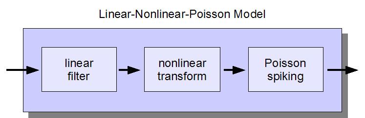
There are three stages of the LNP cascade model. The first stage consists of a linear filter, or linear receptive field, which describes how the neuron integrates stimulus intensity over space and time. The output of this filter then passes through a nonlinear function, which gives the neuron's instantaneous spike rate as its output. Finally, the spike rate is used to generate spikes according to an inhomogeneous Poisson process.

The linear filtering stage performs dimensionality reduction, reducing the high-dimensional spatio-temporal stimulus space to a low-dimensional feature space, within which the neuron computes its response. The nonlinearity converts the filter output to a (non-negative) spike rate, and accounts for nonlinear phenomena such as spike threshold (or rectification) and response saturation. The Poisson spike generator converts the continuous spike rate to a series of spike times, under the assumption that the probability of a spike depends only on the instantaneous spike rate.

Single-filter LNP

Let x denote the spatio-temporal stimulus vector at a particular instant, and k denote a linear filter (the neuron's linear receptive field), which is a vector with the same number of elements as x . Let f denote the nonlinearity, a scalar function with non-negative output. Then the LNP model specifies that, in the limit of small time bins,

P ( spike ) f ( k x ) .

For finite-sized time bins, this can be stated precisely as the probability of observing y spikes in a single bin:

P ( y ~spikes ) = ( Δ λ ) y y ! e Δ λ where λ = f ( k x ) , and Δ is the bin size.

Multi-filter LNP

For neurons sensitive to multiple dimensions of the stimulus space, the linear stage of the LNP model can be generalized to a bank of linear filters, and the nonlinearity becomes a function of multiple inputs. Let k 1 , k 2 , , k n denote the set of linear filters that capture a neuron's stimulus dependence. Then the multi-filter LNP model is described by

P ( spike ) f ( k 1 x , k 2 x , , k n x )

or

P ( spike ) f ( K x ) ,

where K is a matrix whose columns are the filters k i .

Estimation

The parameters of the LNP model consist of the linear filters { k i } and the nonlinearity f . The estimation problem (also known as the problem of neural characterization) is the problem of determining these parameters from data consisting of a time-varying stimulus and the set of observed spike times. Techniques for estimating the LNP model parameters include:

  • moment-based techniques, such as the spike-triggered average or spike-triggered covariance
  • with information-maximization or maximum likelihood techniques.
  • The LNP model provides a simplified, mathematically tractable approximation to more biophysically detailed single-neuron models such as the integrate-and-fire or Hodgkin–Huxley model.
  • If the nonlinearity f is a fixed invertible function, then the LNP model is a generalized linear model. In this case, f is the inverse link function.
  • An alternative to the LNP model for neural characterization is the Volterra kernel or Wiener kernel series expansion, which arises in classical nonlinear systems-identification theory. These models approximate a neuron's input-output characteristics using a polynomial expansion analogous to the Taylor series, but do not explicitly specify the spike-generation process.
  • References

    Linear-nonlinear-Poisson cascade model Wikipedia